Combining two cell formulas/one with filter function

ChristineJ

Well-known Member
Joined
May 18, 2009
Messages
761
Office Version
  1. 365
Platform
  1. Windows
This formula checks if the cell values in one range match those in another range and returns "yes" if true.
Code:
=IF(SUMPRODUCT(--(AL47:AL59=W1:W13)),"yes","no")

This function in cell W1 returns the values in W1:W13:
Code:
=FILTER(L32:L162,TRIM(J32:J162)="Sales")

I'd like to combine the two so no values actually have to appear in W1:W13. I'm trying the following and getting #NA.
Code:
=IF(SUMPRODUCT(--(AL47:AL59=FILTER(L32:L162,TRIM(J32:J162)="Sales"))),"yes","no")

Can this be done? Thanks.
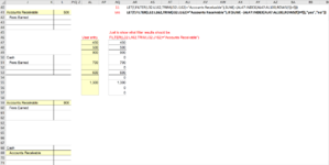
 

Excel Facts

Excel motto
Not everything I do at work revolves around Excel. Only the fun parts.
You will get that error if the filter doesn't return 13 items.
Try
Excel Formula:
=LET(f,FILTER(L32:L162,TRIM(J32:J162)="Sales"),IF(SUM(--(AL47:INDEX(AL47:AL100,ROWS(f))=f)),"yes","no"))
 
Upvote 0
You will get that error if the filter doesn't return 13 items.
Try
Excel Formula:
=LET(f,FILTER(L32:L162,TRIM(J32:J162)="Sales"),IF(SUM(--(AL47:INDEX(AL47:AL100,ROWS(f))=f)),"yes","no"))
 
Upvote 0
Glad to help & thanks for the feedback.
 
Upvote 0
You will get that error if the filter doesn't return 13 items.
Try
Excel Formula:
=LET(f,FILTER(L32:L162,TRIM(J32:J162)="Sales"),IF(SUM(--(AL47:INDEX(AL47:AL100,ROWS(f))=f)),"yes","no"))
I had said that this code was working, but at the time I had only quickly tested it when it should have returned "yes". I'm having trouble getting it to return "no" when the values in the two ranges do not match.

I attached a sample screenshot. (This one filters on "Accounts Receivable" rather than "Sales") where the filter returns 11 rows in the range that should be matched to a user's 11 entries in AL47:AL57.

Your formula is in AQ41. Just the sum of the matches part of your formula is in AQ40, and that number does change if the entries change.

For example, if I change L41 to 5, AQ40 changes to 10 from 11, but "yes" still appears in AQ41. Likewise, if instead I change AL49 to 9.

Nothing I try changes AQ41 to "no".

This is exactly what I need to do; I just can't get it working right! Thanks.
 

Attachments

  • MrExcel.png
    MrExcel.png
    70.8 KB · Views: 5
Upvote 0
Missed a bit out, it should be
Excel Formula:
=LET(f,FILTER(L32:L162,TRIM(J32:J162)="Sales"),IF(SUM(--(AL47:INDEX(AL47:AL100,ROWS(f))=f))=Rows(f),"yes","no"))
 
Upvote 0
Solution
Missed a bit out, it should be
Excel Formula:
=LET(f,FILTER(L32:L162,TRIM(J32:J162)="Sales"),IF(SUM(--(AL47:INDEX(AL47:AL100,ROWS(f))=f))=Rows(f),"yes","no"))
Yes, that works! Thank you so much for following up. CJ
 
Upvote 0
Glad to help & thanks for the feedback.
 
Upvote 0

Forum statistics

Threads
1,214,529
Messages
6,120,070
Members
448,943
Latest member
sharmarick

We've detected that you are using an adblocker.

We have a great community of people providing Excel help here, but the hosting costs are enormous. You can help keep this site running by allowing ads on MrExcel.com.
Allow Ads at MrExcel

Which adblocker are you using?

Disable AdBlock

Follow these easy steps to disable AdBlock

1)Click on the icon in the browser’s toolbar.
2)Click on the icon in the browser’s toolbar.
2)Click on the "Pause on this site" option.
Go back

Disable AdBlock Plus

Follow these easy steps to disable AdBlock Plus

1)Click on the icon in the browser’s toolbar.
2)Click on the toggle to disable it for "mrexcel.com".
Go back

Disable uBlock Origin

Follow these easy steps to disable uBlock Origin

1)Click on the icon in the browser’s toolbar.
2)Click on the "Power" button.
3)Click on the "Refresh" button.
Go back

Disable uBlock

Follow these easy steps to disable uBlock

1)Click on the icon in the browser’s toolbar.
2)Click on the "Power" button.
3)Click on the "Refresh" button.
Go back
Back
Top