compare and find prize through prefix

[Yaseraliakram]

Hi guys

I was wondering if someone could help me with this challenage.
I am looking for a formula to calculate a prize based on the prefix (telephonenumber breakout).
These breakouts are to call international.

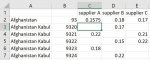
See below the prefix and rate example template.
It works like this, if the prefix is mentioned al the digits after the prefix would be ignored and the rate for the mantion prefix would be charged.
So someone is dialing 932523658923 the rate of 0.1808 would be charged but if someone is calling 937352685984 the rate of 0.1466 woud be charged beceause it prefix is mentioned in the system.

I dont have the prize for all prefixes, so i need to match the prize based on the existing prize.

So in below example they are sorted first on name and then on prefix. (93)
Some of the prefixes can go up to 12 digits.

935 should be 0.1808
9375 should be 0.1691
93702 would 0.1663
933 would be 0.1808

Afghanistan	93​	0.1808​
Afghanistan	935​
Afghanistan Mobile	937​	0.1691​
Afghanistan Mobile	9373​	0.1466​
Afghanistan Mobile AT	9375​
Afghanistan Mobile AWCC	9370​	0.1663​
Afghanistan Mobile AWCC	93702​
Afghanistan	933​

 

[jasonb75]

I'm lost, this just appears to be undoing the work of deleting the rows in your previous thread??

 

[Yaseraliakram]

hahaha, i understand why you are confused, let me explain.

Now the things is as follow,
I have to delete first prefixes which are extra. (this was the previuos post)

Now i have many suppliers whom i am buying from.
I compare with vlookup simple the prize from all supllier based on the prefix. and i can see wich are the chepeast and wich supllier is the most expensive one for each prefix.

Suppliers play a tricky game they give extra prefixes what other suppliers dont have just to be shown as cheapest.

So for example

		supplier A	supplier B	supplier C
Afghanistan	93​	0.1575​	0.18​	0.17​
Afghanistan Kabul	9320​		0.17​
Afghanistan Kabul	9321​	0.22​		0.21​
Afghanistan Kabul	9322​		0.15​	0.22​
Afghanistan Kabul	9323​	0.18​
Afghanistan Kabul	9324​		0.22​

Some supliers give me prefixes with different prizes what other suppliers dont have.
For this i need to formula to get the prizes from missing breakouts, and then i can get a final list. to setup my selling prize to my customers.

so the final file would be like this.

		supplier A	supplier B	supplier C	Most expensive
Afghanistan	93​	0.1575​	0.18​	0.17​	0.18​
Afghanistan Kabul	9320​	0.1575​	0.17​	0.17​	0.17​
Afghanistan Kabul	9321​	0.22​	0.18​	0.21​	0.22​
Afghanistan Kabul	9322​	0.1575​	0.15​	0.22​	0.22​
Afghanistan Kabul	9323​	0.18​	0.18​	0.17​	0.18​
Afghanistan Kabul	9324​	0.1575​	0.22​	0.17​	0.22​

 

[jasonb75]

I've been encountering errors with numbers formatted as text, which I think (and hope) is just the result of copying the sample table from the forum and pasting to excel. If your real data is in the same format then it will be a problem.

I've assumed that the header 'Supplier A' is in C1, the formula and instructions are based on that.

First select columns C:E (entire columns). Next press 'Ctrl g' then click 'Special' choose 'Blanks' and click 'OK'
If done correctly, this should select all of the cells where the price is missing.

Check that the ActiveCell (the selected cell with the lighter background) is in column C, if it is not, use the tab key to move to a cell that is in column C.

Press 'F2' then paste the formula below, followed by 'Ctrl Enter'

=IFERROR(INDEX(C:C,AGGREGATE(15,6,ROW($B$2:$B$7)/($B$2:$B$7=INT(INDIRECT("RC2",0)/({10}^COLUMN($A$1:$M1)))),1)),"")

Hopefully that will do what you need it to.

 

[Yaseraliakram]

I have put in your formula and pressed enter, but there is no value, i just see the formula but no result.

but the cell stays blank, did you had the same problem in The beginning ? (see attachment)

 

[Yaseraliakram]

i see, why this happends,

i put in your formula =IFERROR(INDEX(C:C,AGGREGATE(15,6,ROW($B$2:$B$7)/($B$2:$B$7=INT(INDIRECT("RC2",0)/({10}^COLUMN($A$1:$M1)))),1)),"Failed")

and this is what i get

		supplier A	supplier B	supplier C
Afghanistan	93	0.1575	0.18	0.17
Afghanistan Kabul	9320	Failed	0.17	Failed
Afghanistan Kabul	9321	0.22	Failed	0.21
Afghanistan Kabul	9322	Failed	0.15	0.22
Afghanistan Kabul	9323	0.18	Failed	Failed
Afghanistan Kabul	9324	Failed	0.22	Failed

 

[jasonb75]

Does the formula =ISNUMBER(B2) show TRUE or FALSE?

If it shows FALSE then that is the same problem that I was having. I tried the usual methods of resolution but none of them worked, I had to reproduce the table manually on a blank sheet

 

[Yaseraliakram]

it shows true

 

[jasonb75]

Could you try the same for B3:B7, if any show FALSE then it might cause an error.

Another thing to test would be to select C3, then go to the Formulas tab on the excel ribbon, then click 'Evaluate Formula'
Click the 'Evaluate' button on the popup box 7 times, then capture an image of what is in the box. That stage of calculation is where I identified the problem that I encountered.

 

[Yaseraliakram]

The errors start from step 4. the formula i have used are translated in dutch but they are correct.
=ALS.FOUT(INDEX(C:C,AGGREGAAT(15,6,RIJ($B$2:$B$7)/($B$2:$B$7=INTEGER(INDIRECT("RC2",0)/({10}^KOLOM($A$1:$M1)))),1)),"")