Compare Quantity Ordered against Unique ID in two worksheets/Workbook

[rummaan17]

Dear Members,
I am looking for a routine that can compare the number of quantities requested with the number of quantities ordered against a particular Unique ID.
I am expecting following :
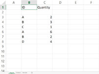
1. Select Unique ID Column and Quantities Column in Base Sheet (Requested) through Input Box.
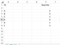
2. Select Unique ID Column and Quantities Column in Ordered sheet through Input box.
3. Add total value against ID before comparing in both sheets.
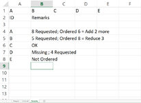
3. Generate another sheet 'Remarks' and report differences in both sheets (As per ID) either as "ADDITIONAL", "REDUCE QUANTITY" OR "NOT AVAILABLE" -

Please see the below screenshots / Excel File to have an idea of what I am trying to achieve.

Any help would be highly appreciated. Thanks a lot

I found some similar code in another website which compares for changes between two sheets 'Yesturday' and 'Today' are report them on new worksheet 'Changes'.

If anyone can edit this routine for the following it would also work :
1. it can take range as Inputbox from different columns in both worksheets so we have the flexibility of comparison without predefined columns.
2. It sum up Quantities under ID before comparison
3. Report difference as in words rather then highlighting as colors.

Option Explicit
Sub CompareYesterdayToday()
Dim wY As Worksheet, wT As Worksheet, wC As Worksheet
Dim c As Range, FR As Long, NR As Long
Dim cc As Long, nc As Long
Application.ScreenUpdating = False
Set wY = Worksheets("Yesterday")
Set wT = Worksheets("Today")
Set wC = Worksheets("Changes")
'1) any item (IDNUMBER) that is in "yesterday" but not in "today"
' should be copied in the worksheet "changes" with the whole row highlighted in red (dropped item).
For Each c In wY.Range("B2", wY.Range("B" & Rows.Count).End(xlUp))
  FR = 0
  On Error Resume Next
  FR = Application.Match(c, wT.Columns(2), 0)
  On Error GoTo 0
  If FR = 0 Then
    NR = wC.Range("B" & wC.Rows.Count).End(xlUp).Offset(1).Row
    wY.Range("A" & c.Row & ":H" & c.Row).Copy wC.Range("A" & NR)
    wC.Range("A" & NR).Resize(, 8).Interior.Color = 255
  End If
Next c
'2) any item (IDNUMBER) that is not in "yesterday" but that is in "today"
' should be copied in the worksheet "changes" with the whole row highlighted in green (new item).
For Each c In wT.Range("B2", wT.Range("B" & Rows.Count).End(xlUp))
  FR = 0
  On Error Resume Next
  FR = Application.Match(c, wY.Columns(2), 0)
  On Error GoTo 0
  If FR = 0 Then
    NR = wC.Range("B" & wC.Rows.Count).End(xlUp).Offset(1).Row
    wT.Range("A" & c.Row & ":H" & c.Row).Copy wC.Range("A" & NR)
    wC.Range("A" & NR).Resize(, 8).Interior.Color = 65280
  End If
Next c
'3) any item (IDNUMBER) that is both in "yesterday" and "today" should only be copied in the worksheet "changes"
' when some cell of the row has been modified (i.e. difference between "yesterday" and "today"), in which case,
' the modified cells should be highlighted in yellow. Ideally, when some changes occured for an item,
' I would like to be able to present both values in the same cell next to each other
' ("yesterday",s value in red and "today"'s value in green).
For Each c In wY.Range("B2", wY.Range("B" & Rows.Count).End(xlUp))
  FR = 0
  On Error Resume Next
  FR = Application.Match(c, wT.Columns(2), 0)
  On Error GoTo 0
  If FR <> 0 Then
    NR = wC.Range("B" & wC.Rows.Count).End(xlUp).Offset(1).Row
    nc = 0
    For cc = 3 To 8 Step 1
      If wY.Cells(c.Row, cc) <> wT.Cells(FR, cc) Then nc = nc + 1
    Next cc
    If nc = 6 Then
      wC.Cells(NR, 1).Resize(, 2).Value = wY.Cells(c.Row, 1).Resize(, 2).Value
      With wC.Cells(NR, 3)
        .NumberFormat = "@"
        .Value = wY.Cells(c.Row, 3).Value & "/" & wT.Cells(FR, 3).Value
      End With
      With wC.Cells(NR, 4)
        .NumberFormat = "@"
        .Value = wY.Cells(c.Row, 4).Value & "/" & wT.Cells(FR, 4).Value
      End With
      With wC.Cells(NR, 5)
        .NumberFormat = "@"
        .Value = wY.Cells(c.Row, 5).Value & "/" & wT.Cells(FR, 5).Value
      End With
      With wC.Cells(NR, 6)
        .NumberFormat = "@"
        .Value = wY.Cells(c.Row, 6).Value & "/" & wT.Cells(FR, 6).Value
      End With
      With wC.Cells(NR, 7)
        .NumberFormat = "@"
        .Value = wY.Cells(c.Row, 7).Value & "/" & wT.Cells(FR, 7).Value
      End With
      With wC.Cells(NR, 8)
        .NumberFormat = "@"
        .Value = wY.Cells(c.Row, 8).Value & "/" & wT.Cells(FR, 8).Value
      End With
      wC.Range("C" & NR).Resize(, 6).Interior.Color = 65535
    ElseIf nc > 0 And nc < 6 Then
      wC.Cells(NR, 1).Resize(, 2).Value = wY.Cells(c.Row, 1).Resize(, 2).Value
      For cc = 3 To 8 Step 1
        If wY.Cells(c.Row, cc) <> wT.Cells(FR, cc) Then
          With wC.Cells(NR, cc)
            .NumberFormat = "@"
            .Value = wY.Cells(c.Row, cc).Value & "/" & wT.Cells(FR, cc).Value
            .Interior.Color = 65535
          End With
        End If
      Next cc
    End If
  End If
Next c
wC.Activate
Application.ScreenUpdating = True
End Sub

EDIT
Also asked here https://www.excelforum.com/excel-pr...unique-id-in-two-worksheets-workbook.html[/I]