Compile data from columns on different sheets into a column in a separate sheet (VBA)

[Allan91]

Hi Guys,

Absolute VBA beginner here. I have been researching to find out how to do the following but to no avail.

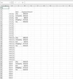
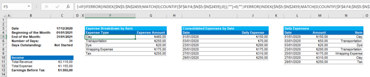
I have created a book with 12 months which has columns containing data.

Please see snapshots I have added. New entries are being added to these lists via index match formulas (Figure 1).

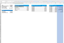
I have been trying to write a VBA code with a command button in order to stack all of the respective data and update the table whenever a new entry is made in a separate sheet (i.e. all months' items in C:C and all months' expenses in D:D in 2 separate columns) and with their relative months in the next column (Figure 2). I need this to create a compiled raw data for my dynamic charts. I have been playing with if statements where I have failed horribly, I mean what I have tried is not even worth to share here unfortunately. I need to have each respective column pasted and with no spaces in between.

This is my first time posting here, I hope I have explained what I have been trying to do clearly enough. I honestly don't know how hard to write a code this requires but I'd be over the moon if you guys could help me with this task.

 

[Norie]

So you want to consolidate the data from columns F&G for each month?

How have you named your sheets? If you have used the month names something like this might work.

Option Explicit

Sub ConsolidateExpenses()
Dim wsMonth As Worksheet
Dim wsNew As Worksheet
Dim rngDst As Range
Dim rngSrc As Range
Dim idxMonth As Long

    Set wsNew = Sheets.Add

    With wsNew
        .Range("C3:D3").Value = Array("Item", "Expense Amount")
        Set rngDst = .Range("C4")
    End With
    
    For idxMonth = 1 To 12
    
        Set wsMonth = Sheets(MonthName(idxMonth, False))
        
        With wsMonth
            Set rngSrc = .Range("F5", .Range("G" & Rows.Count).End(xlUp))
        End With
        
        If rngSrc.Row > 4 Then
            rngSrc.Copy rngDst
            rngDst.Offset(, -1).Resize(rngSrc.Rows.Count) = wsMonth.Name
            Set rngDst = rngDst.Offset(rngSrc.Rows.Count)
        End If
        
    Next idxMonth
    
End Sub

 

[Allan91]

So you want to consolidate the data from columns F&G for each month?

How have you named your sheets? If you have used the month names something like this might work.

Option Explicit

Sub ConsolidateExpenses()
Dim wsMonth As Worksheet
Dim wsNew As Worksheet
Dim rngDst As Range
Dim rngSrc As Range
Dim idxMonth As Long

    Set wsNew = Sheets.Add

    With wsNew
        .Range("C3:D3").Value = Array("Item", "Expense Amount")
        Set rngDst = .Range("C4")
    End With
   
    For idxMonth = 1 To 12
   
        Set wsMonth = Sheets(MonthName(idxMonth, False))
       
        With wsMonth
            Set rngSrc = .Range("F5", .Range("G" & Rows.Count).End(xlUp))
        End With
       
        If rngSrc.Row > 4 Then
            rngSrc.Copy rngDst
            rngDst.Offset(, -1).Resize(rngSrc.Rows.Count) = wsMonth.Name
            Set rngDst = rngDst.Offset(rngSrc.Rows.Count)
        End If
       
    Next idxMonth
   
End Sub

What I actually want to do is consolidating contents of F:F in all 12 sheets (months) on to the F column of a 13th sheet. And the same for G:G. Plus Id like to automatically add the month next to each item.

 

[Norie]

The code I posted kind of does that though it puts the data in columns D & E on a new sheet and the month in column B.

Did you try it?

 

[Allan91]

The code I posted kind of does that though it puts the data in columns D & E on a new sheet and the month in column B.

Did you try it?

I just arrived back home. I was having trouble with tables combined with index match entries. I'll try to fix that first, try your solution and report back. Thank you very much for your help!

 

[Allan91]

The code I posted kind of does that though it puts the data in columns D & E on a new sheet and the month in column B.

Did you try it?

Hey it works!

Though I have 2 problems with it.

1. It also copies the blank cells with it. It's probably because I have the aforementioned index match formulas in the cells.
2. This one is due to my phrasing I know When I said a separate sheet, I actually meant a sheet that already exists and updates as I run the code. One called "Raw Data" actually.

Please see the uploaded image you'll see what I mean.

Thanks a ton Norie!

 

[Norie]

Do you mean that in each tab you have formulas copied down in columns F & G?

P.S. Which uploaded image are you referring to?

 

[Allan91]

Do you mean that in each tab you have formulas copied down in columns F & G?

P.S. Which uploaded image are you referring to?

Sorry I thought I uploaded a new image. I'll upload again

Yes I have formulas copied down to F and G. When I write my expenses somewhere else it sums all the expenses for each item. For example if I bought clay on 2 different dates, it sums them.

 

[Norie]

Can you post an example of the formulas in F and G?

 

[Allan91]

Can you post an example of the formulas in F and G?

Sure thing. I will actually share the whole sheet of January as well. So that you can see all the kind of items I'm trying to copy. I have been trying to expand this for the other items as well but although it does work it gives me a circular reference error as well for some reason.

Please excuse me if the formula is unnecessarily long. I'm a newbie like I said.

This is the formula for 1st item bought. (please see the image)

=IF(IFERROR(INDEX($N$5:$N$2459;MATCH(0;COUNTIF($F$4:F4;$N$5:$N$2459);0));"")=0;"";IFERROR(INDEX($N$5:$N$2459;MATCH(0;COUNTIF($F$4:F4;$N$5:$N$2459);0));""))

On image 1 you can see how this formula works. There's also a simpler one with just sumif for summing the expenses.

On image 2 and 3 you can see the whole sheet for reference. Maybe you'll have a better idea of what I'm trying to accomplish.