complex conditional formatting

[jbrown021286]

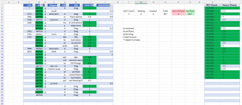
i am building an account tracking spreadsheet. in column D i have the account numbers, in column I is the balance due, column J is balance adjustment amounts, column S is account numbers that have made a payment, and column T is the amount that has been paid on the account. currently i have conditional formatting that highlights when there are matching account numbers in columns D & S and highlights columns I & T if the subsequent balance and payments match. i am wanting to also make it to where the matching criteria takes into account the adjustment in column J and if the sum of I & J equals T then all 5 cells are highlighted. the conditional formatting formulas i currently have are for column D (=$I$2:$I$32,$I$301:$I$311) and (=$D$2:$D$32,$D$301:$D$310) column I (=$I$2:$I$32,$I$301:$I$311) and (=$D$2:$D$32,$D$301:$D$310) column S (=$T$2:$T$55) and (=$S$2:$S$55) column T (=$T$2:$T$55) and (=$S$2:$S$55).

 

[awoohaw]

@jbrown021286 , can you tellme what this formula does: column D (=$I$2:$I$32,$I$301:$I$311) there is no function or operator in there, so I'm confused with the comma. Is this from a different language version of excel?

 

[awoohaw]

Try this, It doesn't compy the blue through all 5 columns you state in your question, but i think you can figure it out. If not just ask.

mr excel questions 17.xlsm
			C	D	E	F	G	H	I	J	K	L	M	N	O	P	Q	R	S	T
1			TAG	RO	??	Daignos	COD	JOB	FLAG TIM	ADJUSTMEN									RO CHECK	Hours Check
2			*	467318	g		d	Diag	1			Don’t Count	Waiting	Incorrect	Total	Not Veriffied	Verified		467318	1
3				467402	g	recall				0.2		3	0	0	36.7	3	29.7		467402	0.2
4			5737	467504	g	alternator	d	Diag	1										467504	1
5			3293	467509	g		ts	Trans service	0.8	0.5									467509	1
6			5740	467520	c	injectors	d	Diag	1										467509	0.3
7			3298	467532	g		rca	ar and camera	3										467532	3
8				467533	g		a	Alignment	1			X=Incorrect							467533	1
9				467605	g		d	Diag	1	0.5		G=Verified							467605	1.5
10			5761	467614	c		d	Diag	1			W=Waiting							467626	2.8
11			5763	467621	*	trans	d	Diag	1			C=Don't Count							467626	1.7
12			1793	467626	g		30k	30k	2.8			*=Need To Check							467638	2.8
13				467626	g		br	turn rotors	1.7										467638	1.7
14				467638	g		ac	ac service	1.5										467641	0.5
15				467638	g		bulb	bulb	0.1										467679	2
16			7844	467640	c	alternator	d	Diag	1										467690	3.8
17			4616	467641	g	tbelt	d	Diag	1	-0.5									467705	0.3
18
Sheet2

Cells with Conditional Formatting
Cell	Condition		Cell Format	Stop If True
I2:I17,T2:T17	Expression	=OR($J2=$T2,$I2+$J2=$T2)	text	NO
D2:D17,S2:S17	Expression	=$D2=$S2	text	NO