Complicated SUMIFS/COUNTIFS Formulas Required

[Chris_010101]

Hello,

I have two sheets, named:

1. Master Data - This sheet will be updated daily by pasting a system report over the existing data
2. 2022 - I want to calculate some stats from the master data sheet on this sheet

The gist of this is, I need to report on people who leave between 0 and 5 months (under 6 months) of employment.

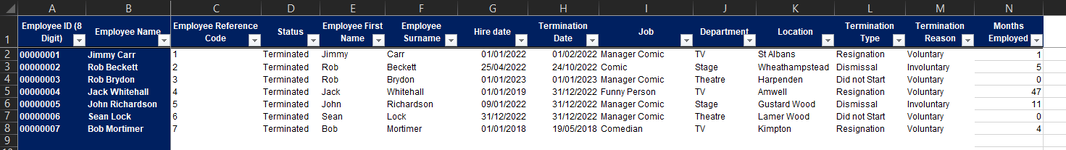
Master Data (Anonymised)

Chris Ops - Attrition Report (ANONYMISED).xlsm
	A	B	C	D	E	F	G	H	I	J	K	L	M	N
1	Employee ID (8 Digit)	Employee Name	Employee Reference Code	Status	Employee First Name	Employee Surname	Hire date	Termination Date	Job	Department	Location	Termination Type	Termination Reason	Months Employed
2	00000001	Jimmy Carr	1	Terminated	Jimmy	Carr	01/01/2022	01/02/2022	Manager Comic	TV	St Albans	Resignation	Voluntary	1
3	00000002	Rob Beckett	2	Terminated	Rob	Beckett	25/04/2022	24/10/2022	Comic	Stage	Wheathampstead	Dismissal	Involuntary	5
4	00000003	Rob Brydon	3	Terminated	Rob	Brydon	01/01/2023	01/01/2023	Manager Comic	Theatre	Harpenden	Did not Start	Voluntary	0
5	00000004	Jack Whitehall	4	Terminated	Jack	Whitehall	01/01/2019	31/12/2022	Funny Person	TV	Amwell	Resignation	Voluntary	47
6	00000005	John Richardson	5	Terminated	John	Richardson	09/01/2022	31/12/2022	Manager Comic	Stage	Gustard Wood	Dismissal	Involuntary	11
7	00000006	Sean Lock	6	Terminated	Sean	Lock	31/12/2022	31/12/2022	Manager Comic	Theatre	Lamer Wood	Did not Start	Voluntary	0
8	00000007	Bob Mortimer	7	Terminated	Bob	Mortimer	01/01/2018	19/05/2018	Comedian	TV	Kimpton	Resignation	Voluntary	4
Master Data

Cell Formulas
Range	Formula
A2:A8	A2	=IF(OR(ISBLANK(C2)), "", REPT(0,8-LEN(C2))&C2)
B2:B8	B2	=IF(OR(ISBLANK(C2)),"",CONCATENATE(E2," ",F2))
N2:N8	N2	=IFERROR(IF(OR(ISBLANK(C2)), "", DATEDIF(G2, H2, "M")), "0")

2022 (Anonymised)

Chris Ops - Attrition Report (ANONYMISED).xlsm
	A	B	C	D	E	F	G	H	I	J	K	L	M
1	2022 - Total Early Churn By Location
2	Location	Jan-22	Feb-22	Mar-22	Apr-22	May-22	Jun-22	Jul-22	Aug-22	Sep-22	Oct-22	Nov-22	Dec-22
3	St Albans
4	Wheathampstead
5	Harpenden
6	Amwell
7	Gustard Wood
8	Lamer Wood
9	Kimpton
10	Total
11
12	2022 - Total Early Churn By Department
13	Department	Jan-22	Feb-22	Mar-22	Apr-22	May-22	Jun-22	Jul-22	Aug-22	Sep-22	Oct-22	Nov-22	Dec-22
14	TV
15	Stage
16	Theatre
17	Total
18
19	2022 - Total Early Churn By Role
20	Role	Jan-22	Feb-22	Mar-22	Apr-22	May-22	Jun-22	Jul-22	Aug-22	Sep-22	Oct-22	Nov-22	Dec-22
21	Manager Comic
22	Comic
23	Funny Person
24	Comedian
25	Total
2022

Cell Formulas
Range	Formula
B10:M10	B10	=IF(SUM(B3:B9)=0, "", SUM(B3:B9))
B25:M25	B25	=IF(SUM(B21:B24)=0,"",SUM(B21:B24))

Stat 1 - total early churn by location

I need to know (numeric) how many people based in location X, who left employment (terminated) in month X (in 2022 only), had between 0 and 5 months employment.

The "total" row is not necessary, just the rows above.

I think stat 2 and 3 I will be ok with as I can amend accordingly, once I have the formula for the above (unless unbeknown to me otherwise!).

Chris

 

[etaf]

does this work for you

location
=COUNTIFS('Master Data'!$N$2:$N$8,"<="&5,'Master Data'!$H$2:$H$8,">="&'2022'!B$2,'Master Data'!$H$2:$H$8,"<="&EOMONTH(B$2,0),'Master Data'!$K$2:$K$8,'2022'!$A3)

department
=COUNTIFS('Master Data'!$N$2:$N$8,"<="&5,'Master Data'!$H$2:$H$8,">="&'2022'!B$13,'Master Data'!$H$2:$H$8,"<="&EOMONTH(B$13,0),'Master Data'!$J$2:$J$8,'2022'!$A14)

role
=COUNTIFS('Master Data'!$N$2:$N$8,"<="&5,'Master Data'!$H$2:$H$8,">="&'2022'!B$20,'Master Data'!$H$2:$H$8,"<="&EOMONTH(B$20,0),'Master Data'!$I$2:$I$8,'2022'!$A21)

Book10
	A	B	C	D	E	F	G	H	I	J	K	L	M
1	2022 - Total Early Churn By Location
2	Location	1/1/22	2/1/22	3/1/22	4/1/22	5/1/22	6/1/22	7/1/22	8/1/22	9/1/22	10/1/22	11/1/22	12/1/22
3	St Albans	0	1	0	0	0	0	0	0	0	0	0	0
4	Wheathampstead	0	0	0	0	0	0	0	0	0	1	0	0
5	Harpenden	0	0	0	0	0	0	0	0	0	0	0	0
6	Amwell	0	0	0	0	0	0	0	0	0	0	0	0
7	Gustard Wood	0	0	0	0	0	0	0	0	0	0	0	0
8	Lamer Wood	0	0	0	0	0	0	0	0	0	0	0	1
9	Kimpton	0	0	0	0	0	0	0	0	0	0	0	0
10	Total		1								1		1
11
12	2022 - Total Early Churn By Department
13	Department	1/1/22	2/1/22	3/1/22	4/1/22	5/1/22	6/1/22	7/1/22	8/1/22	9/1/22	10/1/22	11/1/22	12/1/22
14	TV	0	1	0	0	0	0	0	0	0	0	0	0
15	Stage	0	0	0	0	0	0	0	0	0	1	0	0
16	Theatre	0	0	0	0	0	0	0	0	0	0	0	1
17	Total
18
19	2022 - Total Early Churn By Role
20	Role	1/1/22	2/1/22	3/1/22	4/1/22	5/1/22	6/1/22	7/1/22	8/1/22	9/1/22	10/1/22	11/1/22	12/1/22
21	Manager Comic	0	1	0	0	0	0	0	0	0	0	0	1
22	Comic	0	0	0	0	0	0	0	0	0	1	0	0
23	Funny Person	0	0	0	0	0	0	0	0	0	0	0	0
24	Comedian	0	0	0	0	0	0	0	0	0	0	0	0
25	Total		1								1		1
2022

Cell Formulas
Range	Formula
B3:M9	B3	=COUNTIFS('Master Data'!$N$2:$N$8,"<="&5,'Master Data'!$H$2:$H$8,">="&'2022'!B$2,'Master Data'!$H$2:$H$8,"<="&EOMONTH(B$2,0),'Master Data'!$K$2:$K$8,'2022'!$A3)
B10:M10	B10	=IF(SUM(B3:B9)=0, "", SUM(B3:B9))
B14:M16	B14	=COUNTIFS('Master Data'!$N$2:$N$8,"<="&5,'Master Data'!$H$2:$H$8,">="&'2022'!B$13,'Master Data'!$H$2:$H$8,"<="&EOMONTH(B$13,0),'Master Data'!$J$2:$J$8,'2022'!$A14)
B21:M24	B21	=COUNTIFS('Master Data'!$N$2:$N$8,"<="&5,'Master Data'!$H$2:$H$8,">="&'2022'!B$20,'Master Data'!$H$2:$H$8,"<="&EOMONTH(B$20,0),'Master Data'!$I$2:$I$8,'2022'!$A21)
B25:M25	B25	=IF(SUM(B21:B24)=0,"",SUM(B21:B24))

 

[Chris_010101]

does this work for you

location
=COUNTIFS('Master Data'!$N$2:$N$8,"<="&5,'Master Data'!$H$2:$H$8,">="&'2022'!B$2,'Master Data'!$H$2:$H$8,"<="&EOMONTH(B$2,0),'Master Data'!$K$2:$K$8,'2022'!$A3)

department
=COUNTIFS('Master Data'!$N$2:$N$8,"<="&5,'Master Data'!$H$2:$H$8,">="&'2022'!B$13,'Master Data'!$H$2:$H$8,"<="&EOMONTH(B$13,0),'Master Data'!$J$2:$J$8,'2022'!$A14)

role
=COUNTIFS('Master Data'!$N$2:$N$8,"<="&5,'Master Data'!$H$2:$H$8,">="&'2022'!B$20,'Master Data'!$H$2:$H$8,"<="&EOMONTH(B$20,0),'Master Data'!$I$2:$I$8,'2022'!$A21)

Book10
	A	B	C	D	E	F	G	H	I	J	K	L	M
1	2022 - Total Early Churn By Location
2	Location	1/1/22	2/1/22	3/1/22	4/1/22	5/1/22	6/1/22	7/1/22	8/1/22	9/1/22	10/1/22	11/1/22	12/1/22
3	St Albans	0	1	0	0	0	0	0	0	0	0	0	0
4	Wheathampstead	0	0	0	0	0	0	0	0	0	1	0	0
5	Harpenden	0	0	0	0	0	0	0	0	0	0	0	0
6	Amwell	0	0	0	0	0	0	0	0	0	0	0	0
7	Gustard Wood	0	0	0	0	0	0	0	0	0	0	0	0
8	Lamer Wood	0	0	0	0	0	0	0	0	0	0	0	1
9	Kimpton	0	0	0	0	0	0	0	0	0	0	0	0
10	Total		1								1		1
11
12	2022 - Total Early Churn By Department
13	Department	1/1/22	2/1/22	3/1/22	4/1/22	5/1/22	6/1/22	7/1/22	8/1/22	9/1/22	10/1/22	11/1/22	12/1/22
14	TV	0	1	0	0	0	0	0	0	0	0	0	0
15	Stage	0	0	0	0	0	0	0	0	0	1	0	0
16	Theatre	0	0	0	0	0	0	0	0	0	0	0	1
17	Total
18
19	2022 - Total Early Churn By Role
20	Role	1/1/22	2/1/22	3/1/22	4/1/22	5/1/22	6/1/22	7/1/22	8/1/22	9/1/22	10/1/22	11/1/22	12/1/22
21	Manager Comic	0	1	0	0	0	0	0	0	0	0	0	1
22	Comic	0	0	0	0	0	0	0	0	0	1	0	0
23	Funny Person	0	0	0	0	0	0	0	0	0	0	0	0
24	Comedian	0	0	0	0	0	0	0	0	0	0	0	0
25	Total		1								1		1
2022

Cell Formulas
Range	Formula
B3:M9	B3	=COUNTIFS('Master Data'!$N$2:$N$8,"<="&5,'Master Data'!$H$2:$H$8,">="&'2022'!B$2,'Master Data'!$H$2:$H$8,"<="&EOMONTH(B$2,0),'Master Data'!$K$2:$K$8,'2022'!$A3)
B10:M10	B10	=IF(SUM(B3:B9)=0, "", SUM(B3:B9))
B14:M16	B14	=COUNTIFS('Master Data'!$N$2:$N$8,"<="&5,'Master Data'!$H$2:$H$8,">="&'2022'!B$13,'Master Data'!$H$2:$H$8,"<="&EOMONTH(B$13,0),'Master Data'!$J$2:$J$8,'2022'!$A14)
B21:M24	B21	=COUNTIFS('Master Data'!$N$2:$N$8,"<="&5,'Master Data'!$H$2:$H$8,">="&'2022'!B$20,'Master Data'!$H$2:$H$8,"<="&EOMONTH(B$20,0),'Master Data'!$I$2:$I$8,'2022'!$A21)
B25:M25	B25	=IF(SUM(B21:B24)=0,"",SUM(B21:B24))

Hi There,

Thanks for this.

Unfortunately not, when I add these formulas into my other sheet, where the master data contains about 10,000 rows, it's showing all 0's. I've tried adding 10000 rows in place of 8 on the criteria but this hasn't changed it.

Kind Regards
Chris

 

[Chris_010101]

Hi

Also in your sheet, the months in the header seem to be replaced by dates, 1st Jan to 12 Jan. Could this be a problem?

Unless in American date format?

Kind Regards,
Chris

 

[Chris_010101]

Hey,

I figured it out, thanks so much!!

Chris

 

[etaf]

you are welcome ,
I dont think XL2BB copes very well with dates - when i bring into excel sometimes I get text in US format