Condense a column (by using formula)

[Little_Tiger]

I have 2 columns that is as follow:
A B C D
12 0 6
11 0 4
23 3 3
21 4 8
11 0
10 6
17 0
17 0
28 8
10 0

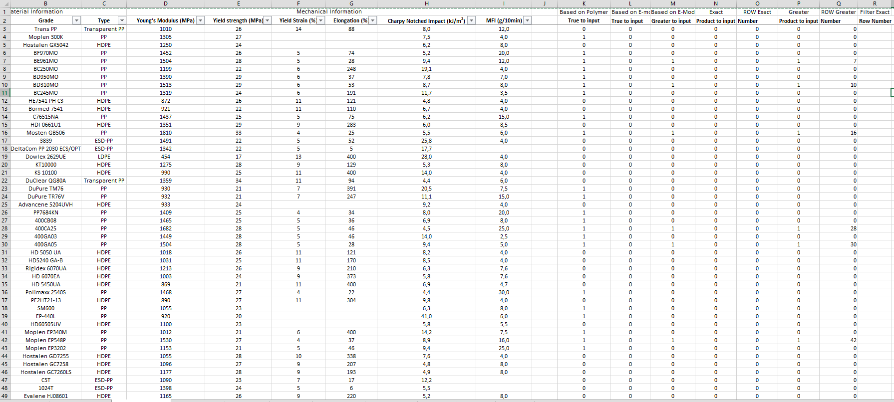
I would like to have in column C, the order from small to large (of column A) based on column B when there is a value greater than 0.
When there is a 0, the formula should ignore and move the the next row. I would like to the formula to condense column B and re-arrange the value in column B based on column A.

Column D shows what I would like to have be done automatically.

Any idea?

thanks, -=LT=-

 

[Rick Rothstein]

Give this array-entered** formula a try...

=IFERROR(VLOOKUP(SMALL(IF(B$1:B$10,A$1:A$10),ROWS($1:1)),A$1:B$10,2,FALSE),"")

**Commit this formula using CTRL+SHIFT+ENTER and not just Enter by itself

 

[Little_Tiger]

Give this array-entered** formula a try...

=IFERROR(VLOOKUP(SMALL(IF(B$1:B$10,A$1:A$10),ROWS($1:1)),A$1:B$10,2,FALSE),"")

**Commit this formula using CTRL+SHIFT+ENTER and not just Enter by itself

Thank for you reply, however not working, it is only return the "".

Here is a real snapshot of the sheet.

Column Q is the column that I Would like to condense in Column R. The order (arranging) of the values in column Q should be based on the values in column D.
Maybe this would help better. Column K to Q are automatically calculated from another sheet. (the Value in column Q are the ROW number where a "search query" give a "1".

 

[Little_Tiger]

 

[Rick Rothstein]

Your original post showed two adjacent columns of data whereas your actual data to be examined is in two widely separated columns, and they start on Row 3, not Row 1... you over simplified your question. Before giving you a formula that will work, I would like you to read something and keep it in mind for future questions you might ask online (whether in this forum or a different one)...

A Generalized "Please Note"
--------------------------------------
For future questions you may ask, please do not simplify your question for us... doing so will get you a great answer to a question you do not actually have and which you do not actually care about AND it will almost always lead to you coming back for help when the solution we give you for the simplified question cannot be applied to your actual data and its layout. One thing you must keep in mind when you ask a question in a forum... the people you are asking to help you know absolutely nothing about your data, absolutely nothing about how it is laid out in the workbook, absolutely nothing about what you want done with it and absolutely nothing about how whatever it is you want done is to be presented back to you as a result... you must be very specific about describing each of these areas, in detail, and you should not assume that we will be able to "figure it out" on our own. Remember, you are asking us for help... so help us to be able to help you by providing the information we need to do so, even if that information seems "obvious" to you (remember, it is only obvious to you because of your familiarity with your data, its layout and the overall objective for it).

Now, as to a formula that should work, give this one a try...

=IFERROR(VLOOKUP(SMALL(IF(Q$3:Q$19,D$3:D$19),ROWS($1:1)),D$3:Q$19,14,FALSE),"")

 

[Little_Tiger]

Your original post showed two adjacent columns of data whereas your actual data to be examined is in two widely separated columns, and they start on Row 3, not Row 1... you over simplified your question. Before giving you a formula that will work, I would like you to read something and keep it in mind for future questions you might ask online (whether in this forum or a different one)...

Now, as to a formula that should work, give this one a try...

=IFERROR(VLOOKUP(SMALL(IF(Q$3:Q$19,D$3:D$19),ROWS($1:1)),D$3:Q$19,14,FALSE),"")

Thank you, it is almost perfect. I 'simplied' it, so I can understand how the formula works. I don't like to just copy paste.
This one work, partially. the column size is large than 19. So be able to get it work, next to change the 19 in most columns, is there any other part of the formula I should change.

Let the 14, in the formula I don't quite understand.

 

[Rick Rothstein]

This one work, partially. the column size is large than 19. So be able to get it work, next to change the 19 in most columns, is there any other part of the formula I should change.

Sorry, I forgot to tell you to change all of the 19's to the row number of your last data element.

Let the 14, in the formula I don't quite understand.

The 14 remains... that is the number of columns Column Q is offset from Column D... the VLOOKUP function needs to know that in order to return the results you want.

 

[Little_Tiger]

Sorry, I forgot to tell you to change all of the 19's to the row number of your last data element.




The 14 remains... that is the number of columns Column Q is offset from Column D... the VLOOKUP function needs to know that in order to return the results you want.

thank you, now I understand. thanks for the help.

 

[Little_Tiger]

Sorry, I forgot to tell you to change all of the 19's to the row number of your last data element.




The 14 remains... that is the number of columns Column Q is offset from Column D... the VLOOKUP function needs to know that in order to return the results you want.

1. There is one more issue. It is a search results, if there is only 1 option. So, who Q column is 0 except for 1 cell, the formula doesn't retrieve that cell in the next column. Do you have any idea why not?

2. Also, if the search is close to the value in column D , (like -10 close) the formula again doesn't pick it up. In column Q everything shows up and works good. However, the formula for R column doesn't retrieve the cell in column Q if the value in column D has a different between -10 or 0. Any idea why this is happening.

I'm trying to solve, try to change my first formula, it still won't.
Picture below shows point number 1. I should expect in column R3 = 16.

 

[Little_Tiger]

1. There is one more issue. It is a search results, if there is only 1 option. So, who Q column is 0 except for 1 cell, the formula doesn't retrieve that cell in the next column. Do you have any idea why not?

2. Also, if the search is close to the value in column D , (like -10 close) the formula again doesn't pick it up. In column Q everything shows up and works good. However, the formula for R column doesn't retrieve the cell in column Q if the value in column D has a different between -10 or 0. Any idea why this is happening.

I'm trying to solve, try to change my first formula, it still won't.
Picture below shows point number 1. I should expect in column R3 = 16.

This was solved. However, I do have a different issue. And I have worked and tried for a week to solve it but I can't.
Anyone who can help me?

As you can see, the latest formula works. However, for certain results it still takes 0 (the orange cells) in the re-ordering of the rows. And also it brings same value more than 1 (green cells).
Anyone would know why this is happening? It doesn't happen for ALL search results, but for a few. (Search is based on NUMBERs).

thanks
-=LT=-