Condition formating with a lot of dates?

[Garfield10]

Hello,
I hope this doesn't sound confusing, but here's my issue.
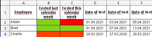
I have a big database structured like this:

In our country, we as a company are forced to test for COVID at least once a week. We have over 1000 employees and you can imagine this would be hell to keep track of manually.
I need Excel to check every name and their respective dates of tests and color the 2 columns appropriately.

I managed to make a formula to check if employee has been tested within past 7 days, but I can't make the calendar week work...

Any help MUCH appreciated!

 

[Garfield10]

Here it's with row/column numbers for convenience... my bad that I didn't realize it.
Thanks to anyone!

 

[Joe4]

Welcome to the Board!

Take a look at the WEEKNUM function, which returns the week number of any date.
You could use this, in conjunction with the YEAR function, to see if a certain date falls within the same year and weeknumber as the current date, i.e.

=AND(WEEKNUM(C2)=WEEKNUM(TODAY()),YEAR(C2)=YEAR(TODAY()))

 

[Garfield10]

Welcome to the Board!

Take a look at the WEEKNUM function, which returns the week number of any date.
You could use this, in conjunction with the YEAR function, to see if a certain date falls within the same year and weeknumber as the current date, i.e.

=AND(WEEKNUM(C2)=WEEKNUM(TODAY()),YEAR(C2)=YEAR(TODAY()))

Hello!

I apologize, I'm really a noob in Excel. I tried this one and it doesn't give me the results I'd need.

Just for certainty, I'll explain again what I need.

Let's take the first employee, Adam. I want to check all his dates when he was tested, so that's 1st, 3rd and 5th of April.
If I had a working formula, Adam would only be highlighted in the "Tested last week" column, as 5th of April still lies in previous week on Monday.

Could you maybe help me a bit more in case I'm just not understanding your formula?

Many thanks, I really appreciate it!

 

[Joe4]

If you wanted to see if he was tested LAST week, then you would need to subtract one from the weeknumber, i.e.

=AND(WEEKNUM(C2)=WEEKNUM(TODAY())-1,YEAR(C2)=YEAR(TODAY()))

The only time this probably won't work well is when you are in the first week of a year, so last week is actually last year.

 

[Garfield10]

If you wanted to see if he was tested LAST week, then you would need to subtract one from the weeknumber, i.e.

=AND(WEEKNUM(C2)=WEEKNUM(TODAY())-1,YEAR(C2)=YEAR(TODAY()))

The only time this probably won't work well is when you are in the first week of a year, so last week is actually last year.

I probably see what you mean now. It works if I select a specific cell, then it tells me e.g. if it's within this week or not when I use this: =AND(WEEKNUM(D2)=WEEKNUM(TODAY()),YEAR(D2)=YEAR(TODAY()))

But that only works for one specific selected date, is there a way to have a formula that checks the whole row, for example D2:D100 and if anywhere in that range there's a date within last or current week, it would color the cell in "Tested last/current week column". I apologize if I make this more confusing that it needs to be, but please don't hesitate to ask if I should explain it in a different way.

I really appreciate your help, this is so important for me to solve... Thank you!

 

[Joe4]

But that only works for one specific selected date, is there a way to have a formula that checks the whole row, for example D2:D100 and if anywhere in that range there's a date within last or current week, it would color the cell in "Tested last/current week column". I apologize if I make this more confusing that it needs to be, but please don't hesitate to ask if I should explain it in a different way.

You are treating each row separately, right?
Meaning that you are conditional formatting each row based ONLY on the data in that particular row, not the other rows right?

If you want to apply a Conditional Formatting formula rule to a whole range at once, first select the whole area that you want to apply it to, and then write the Conditional Formatting formula as it applies to the very first cell in your selection. Excel will adjust it for all the other ones.

So, if you wanted to apply this to cells D2:D100, you would first select the range D2:D100, and then enter the CF formula:

=AND(WEEKNUM(D2)=WEEKNUM(TODAY()),YEAR(D2)=YEAR(TODAY()))

Note how the range references in the formula match the first cell in your selected range.

 

[Garfield10]

Okay, a few points:

1) You are right, I treat each row separately as each row only contains the respective employee's dates of tests.
2) I understand how you meant your last response. I set up a separate rule for last week color and for current week, and yes, it works, now all the dates within last or current week have their respective colors.

however, you probably missed my original intent - if you take a look at the picture I enclosed... it would be much more convenient for me and my colleagues if only the 2 columns with "Tested last week" and "Tested current week" would be colored. Do you get what I mean? Like, I would like to apply the CF only to those 2 columns. The testing dates themselves don't need to be colored. They would only serve as a source for those 2 columns.



English isn't my first language and I'm trying my best to explain it as best as possible, so I apologize if it isn't clear.

I would be over the moon if you managed to help me with this as well... thank you in advance!

 

[Joe4]

however, you probably missed my original intent - if you take a look at the picture I enclosed... it would be much more convenient for me and my colleagues if only the 2 columns with "Tested last week" and "Tested current week" would be colored. Do you get what I mean? Like, I would like to apply the CF only to those 2 columns. The testing dates themselves don't need to be colored. They would only serve as a source for those 2 columns.

No, I got that. Note what I said here:

If you want to apply a Conditional Formatting formula rule to a whole range at once, first select the whole area that you want to apply it to, and then write the Conditional Formatting formula as it applies to the very first cell in your selection. Excel will adjust it for all the other ones.

You only select the ranges that you want the Conditional Formatting to apply to! So it will only be applied to whatever range you selected.

So, only select column B when you create the "last week" conditional formatting rule, and only that column will be colored.
And only select column C when you create the "this week" conditional formatting rule, and only that column will be colored.

 

[Garfield10]

I have Excel 2010. Could it be the cause that I don't know how to first select the area and then apply CF to the B and C column?

Either way, another person responded to me on another forum (I posted here and on the other one in hopes at least someone would help) with this solution:
For last week: =COUNTIFS(B2:ZZ2,">="&TODAY()-WEEKDAY(TODAY(),2)-6,B2:ZZ2,"<="&TODAY()-WEEKDAY(TODAY(),2))
For current week: =COUNTIF(B2:ZZ2,">="&TODAY()-WEEKDAY(TODAY(),2)+1

which works also perfectly...

Nonetheless, I wanted to thank you so much again for your time. Hopefully somebody else will find this topic helpful as well in the future!