Condition formatting rule based on colour or number in another cell that already has a formula (without code)

Woodpusher147

Board Regular
Joined
Oct 6, 2021
Messages
69
Office Version
  1. 365
Platform
  1. Windows
HI all
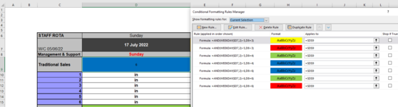
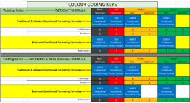
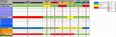
I have a Rota sheet that needs to change cells in D9 and D16 to red if not enough staff, Yellow if minimum, Green if perfect, Blue if too many
This changes on different days.
I have done this by using a simple conditional formatting rule
1658240451708.png

Sunday below is a Black day so simply 6 however there are days that have 4 as perfect and 3 as min so this is the rule I have for those
1658240535938.png


I then have a formula which reads the staff cells D10-D15 & D17-D22 and counts the number of cells containing "in" =SUM(INDEX($O$7:$O$12,MATCH(D10:D15,$N$7:$N$12,0)))

1658240280897.png


At the moment, I have to manually add the conditional formatting to each days D9 and D16 cell.
My question is.
Is it possible to have the relevant conditional formatting rule be auto-populated depending on the colour or number of the DAY cell D7 without going into VBA code

My guess is no as this would need the formula in those cells to change but you guys know much more than me :) maybe an IF cell D7 is ? then use * formatting etc . ?? :/


Thanks for any help
 

Excel Facts

What did Pito Salas invent?
Pito Salas, working for Lotus, popularized what would become to be pivot tables. It was released as Lotus Improv in 1989.
I'm not at all sure that I understand just what you want - but tweaking this should get you to where you want to be.
MrExcelPlayground10.xlsx
D
7Sunday, May 8, 2022
86
9in
10in
11in
12in
13in
14in
154
16in
17lieu
18lieu
19in
20in
21in
Sheet17
Cell Formulas
RangeFormula
D8,D15D8=COUNTIF(D9:D14,"in")
Cells with Conditional Formatting
CellConditionCell FormatStop If True
D8,D15Expression=AND(WEEKDAY($D$7,2)>5,D8=3)textNO
D8,D15Expression=AND(WEEKDAY($D$7,2)>5,D8<3)textNO
D8,D15Expression=AND(WEEKDAY($D$7,2)>5,D8=4)textNO
D8,D15Expression=AND(WEEKDAY($D$7,2)>5,D8>4)textNO
D8,D15Expression=AND(WEEKDAY($D$7,2)<6,D8>6)textNO
D8,D15Expression=AND(WEEKDAY($D$7,2)<6,D8=6)textNO
D8,D15Expression=AND(WEEKDAY($D$7,2)<6,D8<6)textNO
 
Upvote 0
I'm not at all sure that I understand just what you want - but tweaking this should get you to where you want to be.
MrExcelPlayground10.xlsx
D
7Sunday, May 8, 2022
86
9in
10in
11in
12in
13in
14in
154
16in
17lieu
18lieu
19in
20in
21in
Sheet17
Cell Formulas
RangeFormula
D8,D15D8=COUNTIF(D9:D14,"in")
Cells with Conditional Formatting
CellConditionCell FormatStop If True
D8,D15Expression=AND(WEEKDAY($D$7,2)>5,D8=3)textNO
D8,D15Expression=AND(WEEKDAY($D$7,2)>5,D8<3)textNO
D8,D15Expression=AND(WEEKDAY($D$7,2)>5,D8=4)textNO
D8,D15Expression=AND(WEEKDAY($D$7,2)>5,D8>4)textNO
D8,D15Expression=AND(WEEKDAY($D$7,2)<6,D8>6)textNO
D8,D15Expression=AND(WEEKDAY($D$7,2)<6,D8=6)textNO
D8,D15Expression=AND(WEEKDAY($D$7,2)<6,D8<6)textNO
Thank you for the reply and apologies I'm not very clear :/

I have it counting the INs fine but although your way looks much easier than my list of words and the formula =SUM(INDEX($O$7:$O$12,MATCH(D10:D15,$N$7:$N$12,0)))

I will try and be more clear.

Sat - SUn = BLack
Weekdays = Amber
Special days = Red

If its a black day then 6 is the optimal staff and 6 is the min staff
If its an amber day then 4 is the optimal staff and 3 is the min staff

I need the cell in D9 and D16 to shaw the number of staff (in) and change color accordingly as the conditional rules above

The tricky part is, can I apply these rules based on the colour of D7 which would be set depending on day or special day to BLACK/AMBER or RED

HOpe that's clear although I'm not sure :)
 
Upvote 0
You can't change (without VBA) based on the color of the cell. But you can change it based on the reasons why the color would be different. The weekday function will tell you if it's a weekend or weekday. I've put that bit in based on D7. The thresholds change if D7 is a weekday.

Holidays are trickier. You can maintain a list of holidays on your spreadsheet somewhere and check that list.

The formulas get longer and you have more conditions, but all of it can be done.
OK thanks

HOw would the conditional expression formula look for 2 variants i.e. weekday weekend?
And would I simply need to replace the formulas completely if it was a bank holiday
 
Upvote 0
My first response shows how it aught to be for weekday vs weekend on the conditional formatting.

For Bank holidays, you would just search for the date in question on a list of bank holidays, if there was a match, then you'd do a third criteria.
 
Upvote 0
My first response shows how it aught to be for weekday vs weekend on the conditional formatting.

For Bank holidays, you would just search for the date in question on a list of bank holidays, if there was a match, then you'd do a third criteria.
THanks again for the reply
I have implemented the solution but im afraid I cant get it to work.
1658306850636.png

D9 should be green according to the conditional formatting. Also, if I change the date to test it works for weekdays, the cell just turns white

Thanks again for any help
 

Attachments

  • 1658306443504.png
    1658306443504.png
    49.4 KB · Views: 7
Upvote 0
IF we were to use VBA to create the rule based on colour, would that be easier?
If so, would you know how to do this?

Thanks
 
Upvote 0
You'll get it with conditional formatting only.

You have weekday>6 on some of them It aught to be <6 - for the weekdays instead of the weekends. That should settle the rest.

They way you have the formulas in there - you're having two true conditions, so excel will make a choice that's probably not what you would make.
OK Ive changed my mistake ><. ITs now just like your example so not sure what you mean by "They way you have the formulas in there - you're having two true conditions, so excel will make a choice that's probably not what you would make" ?

It appears to be working but may be the wrong way round. If I change the date to a weekday the 6 changes to green which would be right for the weekend. Here is the KEY
1658320179069.png

and here is the full sheet
1658320117559.png


I cant see how to share the actual sheet which Im sure would be helpful.
Once again, thanks for you time
 

Attachments

  • 1658319595137.png
    1658319595137.png
    55.6 KB · Views: 8
  • 1658319629643.png
    1658319629643.png
    41.5 KB · Views: 7
Last edited:
Upvote 0

Forum statistics

Threads
1,214,827
Messages
6,121,806
Members
449,048
Latest member
greyangel23

We've detected that you are using an adblocker.

We have a great community of people providing Excel help here, but the hosting costs are enormous. You can help keep this site running by allowing ads on MrExcel.com.
Allow Ads at MrExcel

Which adblocker are you using?

Disable AdBlock

Follow these easy steps to disable AdBlock

1)Click on the icon in the browser’s toolbar.
2)Click on the icon in the browser’s toolbar.
2)Click on the "Pause on this site" option.
Go back

Disable AdBlock Plus

Follow these easy steps to disable AdBlock Plus

1)Click on the icon in the browser’s toolbar.
2)Click on the toggle to disable it for "mrexcel.com".
Go back

Disable uBlock Origin

Follow these easy steps to disable uBlock Origin

1)Click on the icon in the browser’s toolbar.
2)Click on the "Power" button.
3)Click on the "Refresh" button.
Go back

Disable uBlock

Follow these easy steps to disable uBlock

1)Click on the icon in the browser’s toolbar.
2)Click on the "Power" button.
3)Click on the "Refresh" button.
Go back
Back
Top