Conditional format

tf37

Board Regular
Joined
Apr 16, 2004
Messages
169
Been looking through the help for conditional formatting of cells, and just can't seem to find what I'm after...or perhaps what I'm after isn't possible with conditional format
Have a spread sheet that has row1 with receipt numbers, and the row2 below is amounts. This is used between two different locations.
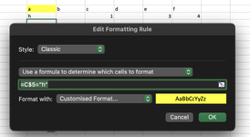
Say location 1 is where I'm at and to let location 2 know that the receipt in row 1 was entered here, I put the letter h in the amount cell (row 2) and highlight row 1 receipt number yellow
Entered in A2 is =A3>0 and conditional format for row a2:l2 is to turn the cell color to yellow.
The cells that they would enter would contain their dollar amounts entered, and should leave the receipt row 1 number with a no fill color.
Is it possible with conditional formatting, or better handled with a "if then" type VBA coding?
Hope that makes sense - thanks
 

Excel Facts

Excel Can Read to You
Customize Quick Access Toolbar. From All Commands, add Speak Cells or Speak Cells on Enter to QAT. Select cells. Press Speak Cells.
JW DC Receipt Totals-conditional.xlsb
ABCDEFGHIJKLM
21765117652176531765417655176561765717658176591766017661176627.00
3 h 5.00-2.00-7.00
4176631766417665176661766717668176691767017671176721767317674
5 h h -
6176751767617677176781767917680176811768217683176841768517686
7-
8176871768817689176901769117692176931769417695176961769717698
9-
10176991770017701177021770317704177051770617707177081770917710
11-
Daily
Cell Formulas
RangeFormula
M2M2=SUM(M3:M55)
M3,M11,M9,M7,M5M3=SUM(A3:L3)
 
Upvote 0
JW DC Receipt Totals-conditional.xlsb
ABCDEFGHIJKLM
21765117652176531765417655176561765717658176591766017661176627.00
3 h 5.00-2.00-7.00
4176631766417665176661766717668176691767017671176721767317674
5 h h -
6176751767617677176781767917680176811768217683176841768517686
7-
8176871768817689176901769117692176931769417695176961769717698
9-
10176991770017701177021770317704177051770617707177081770917710
11-
Daily
Cell Formulas
RangeFormula
M2M2=SUM(M3:M55)
M3,M11,M9,M7,M5M3=SUM(A3:L3)
I think this is what you need
 

Attachments

  • Untitled3.png
    Untitled3.png
    142.9 KB · Views: 12
Upvote 0
How simple...and I tried that but left out the " " - I'll learn someday....perhaps...lol Thank you very much
 
Upvote 0

Forum statistics

Threads
1,214,642
Messages
6,120,698
Members
448,979
Latest member
DET4492

We've detected that you are using an adblocker.

We have a great community of people providing Excel help here, but the hosting costs are enormous. You can help keep this site running by allowing ads on MrExcel.com.
Allow Ads at MrExcel

Which adblocker are you using?

Disable AdBlock

Follow these easy steps to disable AdBlock

1)Click on the icon in the browser’s toolbar.
2)Click on the icon in the browser’s toolbar.
2)Click on the "Pause on this site" option.
Go back

Disable AdBlock Plus

Follow these easy steps to disable AdBlock Plus

1)Click on the icon in the browser’s toolbar.
2)Click on the toggle to disable it for "mrexcel.com".
Go back

Disable uBlock Origin

Follow these easy steps to disable uBlock Origin

1)Click on the icon in the browser’s toolbar.
2)Click on the "Power" button.
3)Click on the "Refresh" button.
Go back

Disable uBlock

Follow these easy steps to disable uBlock

1)Click on the icon in the browser’s toolbar.
2)Click on the "Power" button.
3)Click on the "Refresh" button.
Go back
Back
Top