CONDITIONAL FORMATTING AFTER EVERY CHANGE (across all rows)

[JuicyMusic]

Hello Guru's, I'm stumped. My conditional kind of works but not all the time. Please help.

I have a small set of data with 3 columns on it. I need the conditional formatting to go across all the 3 columns based on a conditional formula in Column B.
I need the conditional formatting to be in column starting in cell B2.

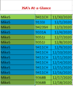
The first row will always be green across all three columns. Green will be the initial color formatting.
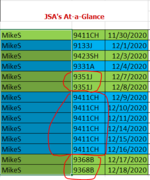
Blue at the 2nd job number change - then back to green at the 3rd change in the job number. Back and forth like that for the length of the data.

1) If the job number in consequent rows are the same, then that cell should be green as well (column A and C of that row should be green as well). Could be the same for several rows. Same color then.
2) At the next job number change, the color for that cell should be blue (columns A and C of that row should be blue as well)….

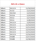
I will attach a clean set of data and a set of data showing the correct color so you can see what the results should be. I'm doing this in case I'm not clear for you.

Column A: employee name
Column B: job number
Column C: date worked on job

Specifics:
Column C: The date order is the first sort. It is from older to newest date. It has to be that way.
Column B: This job number are sorted so that all the "like" job numbers are together from smaller to bigger


Thank you so much!

 

[jasonb75]

This works with a quick test,

=NOT(MOD(ROWS(UNIQUE($B$2:$B2)),2))

 

[JuicyMusic]

I'll try it right now. Give me a sec to try.

 

[JuicyMusic]

Okay, I tried it. It work only in column B. Can you adjust the formula so that the green color highlights in column A and C as well.

Also, I don't see how this formula Blue.
The first block of data should be green - then blue at the next job number change. I think you are sooooo close

 

[JuicyMusic]

Hello Jason, I wanted to add that the first color will always be green - whatever color cell b2 is should be extended to cell A2 and C2.

The color should change at the next job number change.

Example: If there are 5 rows with the same job number - then the color in column A and C or those exact rows should be the same color.

The color coding will be Green, Blue, Green, Blue, etc. etc...…Thank you!!!! I added a snapshot for you.

 

[jasonb75]

It work only in column B. Can you adjust the formula so that the green color highlights in column A and C as well.

It works with any column that you apply it to.

Also, I don't see how this formula Blue.
The first block of data should be green

In your first post, you said

Green will be the initial color formatting.

which implies that the green will be the default colour (manually filled to all cells without conditional formatting).

The formula that I provided for conditional formatting will change the default green to blue for the 2nd, 4th, 6th, etc job numbers.

 

[etaf]

I have taken
Hope jasonb75 does not mind, apologies if you do
I had been looking at a few different solutions , but jasonb75 is the best , as you have a version that supports
and then tested if 0 and 1 to choose green or blue
slight change

jasonb75​

Formula , and so zero = green and 1 = blue

BAND Groups COND-FRMT.xlsx
	A	B	C
2		1
3		1
4		1
5		2
6		3
7		4
8		5a
9		5a
10		6a
11		6a
12		6a
13		7
14		7
15		7
16		7
17		12
Sheet1

Cells with Conditional Formatting
Cell	Condition		Cell Format	Stop If True
A2:C20	Expression	=AND($B2<>"",MOD(ROWS(UNIQUE($B$2:$B2)),2)=0)	text	NO
A2:C20	Expression	=AND($B2<>"",MOD(ROWS(UNIQUE($B$2:$B2)),2)=1)	text	NO

 

[JuicyMusic]

Thank you to Jason....and to you Etaf. I'm trying this right now. Be back.

 

[jasonb75]

Hope jasonb75 does not mind, apologies if you do

Not at all, Wayne! Saves me having to set up an example again

I keep forgetting to save my test files before closing the lid on my laptop and then losing them when it decides to crash (frequently).

 

[etaf]

I keep forgetting to save my test files before closing the lid on my laptop and then losing them when it decides to crash (frequently).

Thanks

I do the same, not crashing, but I delete the spreadsheets and don't save - at least i can get them back copying the XL2BB entry , so not all lost