CONDITIONAL FORMATTING AFTER EVERY CHANGE (across all rows)

[JuicyMusic]

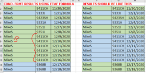
Hello Guru's, I'm stumped. My conditional kind of works but not all the time. Please help.

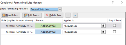
I have a small set of data with 3 columns on it. I need the conditional formatting to go across all the 3 columns based on a conditional formula in Column B.
I need the conditional formatting to be in column starting in cell B2.

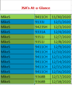
The first row will always be green across all three columns. Green will be the initial color formatting.
Blue at the 2nd job number change - then back to green at the 3rd change in the job number. Back and forth like that for the length of the data.

1) If the job number in consequent rows are the same, then that cell should be green as well (column A and C of that row should be green as well). Could be the same for several rows. Same color then.
2) At the next job number change, the color for that cell should be blue (columns A and C of that row should be blue as well)….

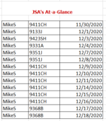
I will attach a clean set of data and a set of data showing the correct color so you can see what the results should be. I'm doing this in case I'm not clear for you.

Column A: employee name
Column B: job number
Column C: date worked on job

Specifics:
Column C: The date order is the first sort. It is from older to newest date. It has to be that way.
Column B: This job number are sorted so that all the "like" job numbers are together from smaller to bigger


Thank you so much!

 

[JuicyMusic]

Here are my results after inserting your two formulas into the Conditional Formatting box, or whatever it's called

My results will be an image because my company doesn't allow me to use Xlb2bb. WE ARE SOOOOO CLOSE!!!

 

[JuicyMusic]

It looks like something happens at row 8. I hope you guys are still here.

 

[etaf]

show use the range in the photo, columns and the rows, I can just see them
Then also post the 2 formulas you have used in the conditional format rules and what colour is used for which formula

=AND($B2<>"",MOD(ROWS(UNIQUE($B$2:$B2)),2)=0) =BLUE
=AND($B2<>"",MOD(ROWS(UNIQUE($B$2:$B2)),2)=1) = green

and the range selected in the conditional formatting
$A$2:$C$100 ???

A screen shot will do

 

[JuicyMusic]

Sirs, please forgive me. I tried on a different set of data from the same spreadsheet and the color coding work perfectly. You guys are awesome!!


Here is the box you requested.

 

[etaf]

excellent , glads its resolved

 

[JuicyMusic]

Sirs, I know my question has been answered but I wanted to add that I think I can tell why what you provided me worked on one set of data but not the other.

I LOVE that fact that I don't have to color code the first row of data manually. Thank you for that.

The CF works perfectly as long as Column B (job number) is in order, ascending or descending. My data set was sorted by Column C (date column) and so the color coding would be off lower down in the data set somewhere.

Let me know if I am correct or if it just looks like this is what is happening to me. Please let me know so I know going forward.

Thank you so much.
Juicy,

 

[etaf]

in your screen show, its only the job numbers that are unique and change colour - so the colour would go off, as the job numbers would go out of order
so if the job numbers happen to be sorted like below , then in order to maintain the changing colour - the job numbers would be different colours -

is this what is happening

1 - green
1 - green
2 - blue
2 - blue
3 - green
1 - blue
2 - green

 

[JuicyMusic]

Yes, that is exactly what is happening. Once I sorted by the job number column the color coding "offness" no longer occurred,

 

[etaf]

the problem nw is you no longer have the grouping.
I'm not sure how to change the colour without perhaps helper columns, which I had googled in the beginning - I would have to repeat and see if i can rethink, hopefully other members may see a solution

how about this example/tutorial to add a helper column - see to have worked

An Excel conditional format that expands with grouped data | TechRepublic

By adding a helper column and a simple conditional format rule, you can apply an alternating band scheme that expands to accommodate a group.

www.techrepublic.com

 

[jasonb75]

Using Wayne's example from post 17, would you want all identical job numbers to be the same colour regardless of order? Note that this would mean that there could be times when there are 2 different job numbers next to each other using the same colour.