Conditional Formatting based cell value

[EMcK01]

Hi,

I want to use the conditional formatting to highlight key dates based on date entered in a cell.

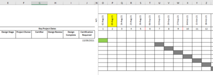
ie. on the image I've uploaded, the date in cell J8 is 13/09/21; I would like to find the corresponding date in the table and fill the cell on row 8 directly below the date in cell J8, column U in this instance. However it is highlighted in column O.

Within conditional formatting I was using "use a formula to determine which cells to format" with the following =MATCH(J8,O5:Z5,0) and applying to O8:Z8

Any suggestions of how to update this to highlight the cell directly below the date I've entered in J8?

Thanks

 

[Fluff]

Try

=$J8=O$5

 

[EMcK01]

Perfect Fluff, thanks for that

 

[Fluff]

You're welcome & thanks for the feedback.