Conditional formatting - cell equals another cell, formats range of cells - quick apply to multiple ranges needed

Robisbald

New Member
Joined
Jun 29, 2022
Messages
6
Office Version
  1. 365
  2. 2016
Platform
  1. Windows
Okay, so whether this is done by VBA or the conditional formatting tool isn't important to me, either would be fine. But at the moment I'm adding each rule manually in the conditional formatting tool and I've got about 200 of these to do and I know an expert out there has an easy solution for this ;)

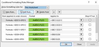
So as an example (and seen on the image attached), I want cells B11:G11 to have the interior colour changed to green when cells D11 & F11 equal each other. But I want this to continue for a specific range of rows below:
when D11=F11 affects B11:G11
when D12=F12 affects B12:G12
when D13=F13 affects B13:G13
when D14=F14 affects B14:G14
when D15=F15 affects B15:G15
note they will be row where I don't want this applying to, so the rows will skip a few before I want the conditional formatting to apply again:
when D20=F20 affects B20:G20
when D21=F21 affects B21:G21
when D22=F22 affects B22:G22

I've tried copy and paste special formatting but this doesn't work, might be doing something wrong, but read that its not great when using a formula based rule?

Thanks
 

Attachments

  • Conditional formatting.PNG
    Conditional formatting.PNG
    17.2 KB · Views: 6

Excel Facts

Difference between two dates
Secret function! Use =DATEDIF(A2,B2,"Y")&" years"&=DATEDIF(A2,B2,"YM")&" months"&=DATEDIF(A2,B2,"MD")&" days"
ok
so i have select contiguous ranges $D$11:$G$15,$D$20:$G$22
for conditional formatting


and also added part of the rule IF D11<>"" then do not apply the colour so info needs to be entered into the cell to work
otherwise a blank = blank and it will colour all empty cells
many different ways to do that

Rule - =AND($D11<>"",$D11=$F11)

Book1
ABCDEFGH
1
2
3
4
5
6
7
8
9
10
11111
122
13
14
1544
16
171212
18
19
2022
21
22
23
24
Sheet3
Cells with Conditional Formatting
CellConditionCell FormatStop If True
D11:G15,D20:G22Expression=AND($D11<>"",$D11=$F11)textNO


Note i used command key to select non-contigous on a Mac
Control key on windows

for 2007, 2010 , 2013 , 2016 , 2019 or 365 Subscription excel version
Conditional Formatting

Highlight applicable range >>
$D$11:$G$15,$D$20:$G$22 - Change, reduce or extend the rows to meet your data range of rows

Home Tab >> Styles >> Conditional Formatting
New Rule >> Use a formula to determine which cells to format
Edit the Rule Description: Format values where this formula is true:
=AND($D11<>"",$D11=$F11)

Format [Number, Font, Border, Fill]
choose the format you would like to apply when the condition is true
OK >> OK
 
Upvote 0
Solution

Forum statistics

Threads
1,214,952
Messages
6,122,454
Members
449,083
Latest member
Ava19

We've detected that you are using an adblocker.

We have a great community of people providing Excel help here, but the hosting costs are enormous. You can help keep this site running by allowing ads on MrExcel.com.
Allow Ads at MrExcel

Which adblocker are you using?

Disable AdBlock

Follow these easy steps to disable AdBlock

1)Click on the icon in the browser’s toolbar.
2)Click on the icon in the browser’s toolbar.
2)Click on the "Pause on this site" option.
Go back

Disable AdBlock Plus

Follow these easy steps to disable AdBlock Plus

1)Click on the icon in the browser’s toolbar.
2)Click on the toggle to disable it for "mrexcel.com".
Go back

Disable uBlock Origin

Follow these easy steps to disable uBlock Origin

1)Click on the icon in the browser’s toolbar.
2)Click on the "Power" button.
3)Click on the "Refresh" button.
Go back

Disable uBlock

Follow these easy steps to disable uBlock

1)Click on the icon in the browser’s toolbar.
2)Click on the "Power" button.
3)Click on the "Refresh" button.
Go back
Back
Top