Conditional formatting for blank cells containing formulas?

[Jyggalag]

Hi all,

I currently have this setup:

I have a row of formulas saying IF(ISBLANK(cell below),return blank value, otherwise return value to the left + 7) to advance the week one week ahead when data is entered.

I want to create a conditional formatting for this row, so whenever a value is entered, it gets highlighted in a certain color.

However, whenever I try this, it highlights all the cells, because they contain this formula (even though the formula returns a blank value, as seen in column G, H and I above for example.

Does anybody know how I can bypass this issue? I hope my question makes sense, otherwise let me know and I would be happy to rephrase!

Kind regards,
Jyggalag

 

[Jamie McMillan]

Hello,

Yes the "" is a 'kind of value'

The conditional formatting formula will be.

=G3=""

Then select no fill - or a different colour.

Jamie

 

[Jyggalag]

Hello,

Yes the "" is a 'kind of value'

The conditional formatting formula will be.

=G3=""

Then select no fill - or a different colour.

Jamie

Hi again Jamie,

I hope that all is well with you. And thank you so much for your quick input

Should I make one conditional formatting rule for each cell (this is fine by the way, as I plan to operate with 4 cells only) then?

I tried this right now, but it does not seem to work (my cell gets highlighted whether there's a value in the cell or not):

 

[Jyggalag]

Hello,

Yes the "" is a 'kind of value'

The conditional formatting formula will be.

=G3=""

Then select no fill - or a different colour.

Jamie

Please disregard my prior question. Your formula worked (just had to use the formula option in conditional formatting).

Apologies and thank you so much Jamie!!

 

[Jamie McMillan]

Hello,

I just posted that before I went out.

In the conditional formatting menu; select "use a formula to determine cells to format". Type in, or paste, =G3="" and choose the format you want.

Then use 'Format Painter' to copy it to all cells. You can type it in to all the cells if you prefer.

Jamie

 

[Jamie McMillan]

Hello Jean,

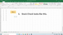
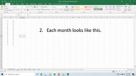
The images below show exactly how the "Test File" should look, and where the values are pasted after the macro runs.

Jamie

 

[Jyggalag]

Hello Jean,

The images below show exactly how the "Test File" should look, and where the values are pasted after the macro runs.

Jamie

Hi Jamie,

I worry that you may have posted this in the wrong thread

BR.
Jyggalag

 

[Jamie McMillan]

HaHaHa,

Yes I Did.

 

[AgingHippie]

What about this option?