mpeterson1227
New Member
- Joined
- Dec 21, 2016
- Messages
- 6
****** id="cke_pastebin" style="position: absolute; top: 0px; width: 1px; height: 1px; overflow: hidden; left: -1000px;">
<tbody style="margin: 0px; padding: 0px; border: 0px;">
</tbody></body>
<tbody style="margin: 0px; padding: 0px; border: 0px;">
</tbody>
Please help and thank you in advance!
| I'm trying to create a formula for conditional formatting that will identify two words and create an output of a word. See example below: 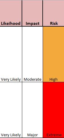
Right now I'm having to manually put in the Risk Type. I want it to output the risk type based on the likelihood and impact. 
|
<tbody style="margin: 0px; padding: 0px; border: 0px;">
</tbody>
| I'm trying to create a formula for conditional formatting that will identify two words and create an output of a word. See example below:
Right now I'm having to manually put in the Risk Type. I want it to output the risk type based on the likelihood and impact.
|
<tbody style="margin: 0px; padding: 0px; border: 0px;">
</tbody>
Please help and thank you in advance!
")


