JAYLEECAKE
New Member
- Joined
- Feb 8, 2021
- Messages
- 4
- Office Version
- 2016
- Platform
- Windows
I am losing my mind over this. I am very well acquainted with Excel; however, this super basic formula is killing me. Have I completely lost it?!
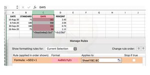
We get a task on certain dates (DATE) and depending on the task, it may either have a 75-day suspense or 180-day suspense (STANDARD).
To find out the number of days the tasker has been active, I calculated the DAYS column with [=DAYS(TODAY(),$A2)]. Works great.
To find out how overdue something is, I calculated the "percent" (though not *100) with [=$C2/$B2]. Works great.
PROBLEM! When I use conditional formatting to highlight in red the cells in PERCENT that are greater than 1 [=$D2>1], it goes wild and highlights Row 2 as well even though $D$2=2.43.
(I will also be adding that if it's greater than or equal to .73 but less than 1 it should be YELLOW. Otherwise, GREEN.)
I have tried this on multiple computers, on brand new spreadsheets, etc. I have tried enclosed IF functions in a separate column to give a RED, GREEN, YELLOW answer, then base the conditional formatting off of that. IT STILL HIGHLIGHTS INCORRECT ROWS! I have no idea what is going on. I feel like I am losing my mind over here...
PLEASE HELP!
Formats: DATE=Date, STANDARD, DAYS, PERCENT all = Number