Conditional formatting help

[Grictori]

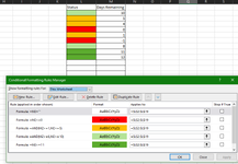
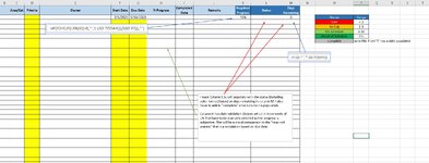
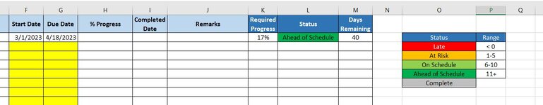
I am trying to add in conditional formatting to a tracker spreadsheet to enter 1 of 4 options from a list based on greater than / less than scenario. Basically, data validation type options, but automated based on days ahead/behind. For example, I have a table/legend that has "late", "at risk", "on schedule", and "ahead of schedule". The criteria is <0, 1-5, 6-10, 10+ respectfully. I also want Red, Orange, light green, and dark green. I have a column on my sheet that calculates how many days from or past the due date as a reference. Can this easily be done?

Thanks for the help

 

[Peter_SSs]

Welcome to the MrExcel board!

I'm a little unsure where some of the category boundaries are (eg whether 10 is in 6-10 or 10+) but could you use formulas like this in the Status column and the conditional formatting as shown?
(I can't tell from the image which columns/rows that data is in so you'll have to adjust)

23 03 07.xlsm
	I	J
1	Status	Days
2	On Schedule	6
3	Ahead of Schedule	25
4
5	Late	-2
6	At Risk	3
Crictori

Cell Formulas
Range	Formula
I2:I6	I2	=IF(J2="","",LOOKUP(J2,{-999,1,6,10},{"Late","At Risk","On Schedule","Ahead of Schedule"}))

Cells with Conditional Formatting
Cell	Condition		Cell Format	Stop If True
I2:I6	Expression	=LEFT(I2,2)="Ah"	text	NO
I2:I6	Expression	=LEFT(I2,2)="At"	text	NO
I2:I6	Expression	=LEFT(I2,2)="La"	text	NO
I2:I6	Expression	=LEFT(I2,2)="On"	text	NO

 

[moddddmyexcel]

Use formula to set your conditional formats. Below is an example. The top rule is just saying if the cell is blank make the color no fill. Keep this at the top to avoid coloring your blanks red.

 

[Grictori]

Ok thanks for the first two responses, but my inexperience is causing me some confusion. I tried your suggestions, but I am doing something wrong. I attached a better image to show what I am trying to accomplish. I hope that clarifies things more. Sorry my work computer will not let me install the add on so I cannot attach the mini-sheet.

 

[Grictori]

Welcome to the MrExcel board!

I'm a little unsure where some of the category boundaries are (eg whether 10 is in 6-10 or 10+) but could you use formulas like this in the Status column and the conditional formatting as shown?
(I can't tell from the image which columns/rows that data is in so you'll have to adjust)

23 03 07.xlsm
	I	J
1	Status	Days
2	On Schedule	6
3	Ahead of Schedule	25
4
5	Late	-2
6	At Risk	3
Crictori

Cell Formulas
Range	Formula
I2:I6	I2	=IF(J2="","",LOOKUP(J2,{-999,1,6,10},{"Late","At Risk","On Schedule","Ahead of Schedule"}))

Cells with Conditional Formatting
Cell	Condition		Cell Format	Stop If True
I2:I6	Expression	=LEFT(I2,2)="Ah"	text	NO
I2:I6	Expression	=LEFT(I2,2)="At"	text	NO
I2:I6	Expression	=LEFT(I2,2)="La"	text	NO
I2:I6	Expression	=LEFT(I2,2)="On"	text	NO

Peter, I am sorry that I am still confused and I appreciate your attempt at helping me. Please see my post below and hopefully it clarifies things more. I am not sure how to make your suggestions work.

 

[Grictori]

Ok thanks for the first two responses, but my inexperience is causing me some confusion. I tried your suggestions, but I am doing something wrong. I attached a better image to show what I am trying to accomplish. I hope that clarifies things more. Sorry my work computer will not let me install the add on so I cannot attach the mini-sheet.

I think I figured it all out. I am now just working on "done" and greying out the entire row if it shows as complete.

 

[Peter_SSs]

I tried your suggestions, but I am doing something wrong. I attached a better image to show what I am trying to accomplish.

I think that my previous suggestion does exactly what you want except that .

1. It was pointed at the wrong columns because we didn't know what they were until post 4, and
2. A new condition/colour has now been introduced.

I think this variation should do what you want. There may be a simpler formula for the status values in column L depending on your new formula in column M. (I am assuming that the formula in column M will change and provide some sort of different result if column I has a date?)

23 03 07.xlsm
	I	J	K	L	M
1	Completed Date			Status	Days
2				On Schedule	6
3				Ahead of Schedule	25
4
5				Late	-2
6				At Risk	3
7
8	7/03/2023			Complete	??
Grictori

Cell Formulas
Range	Formula
L2:L8	L2	=IF(I2="",IF(M2="","",LOOKUP(M2,{-999,1,6,10},{"Late","At Risk","On Schedule","Ahead of Schedule"})),"Complete")

Cells with Conditional Formatting
Cell	Condition		Cell Format	Stop If True
L2:L10	Expression	=LEFT(L2,2)="Co"	text	NO
L2:L10	Expression	=LEFT(L2,2)="Ah"	text	NO
L2:L10	Expression	=LEFT(L2,2)="At"	text	NO
L2:L10	Expression	=LEFT(L2,2)="La"	text	NO
L2:L10	Expression	=LEFT(L2,2)="On"	text	NO

 

[Grictori]

Ok last question and I appreciate all the help. I have everything working thanks to the help except the "complete" function.
Let's say the task is ahead of schedule and I enter a complete date in the "I" column, I want the status to automatically change to "complete".
Right now that status column (Column I) function is only prompted by due date/current date formula.
I believe the formula in the status column conditional formatting is something like =IF($I2>0 but I do not know what the rest should look like. I am also assuming I move this formula up on the priority for conditional formatting?

 

[Peter_SSs]

Let's say the task is ahead of schedule and I enter a complete date in the "I" column, I want the status to automatically change to "complete".
Right now that status column (Column I) function is only prompted by due date/current date formula.

Sounds like you didn't try my last suggestion. It addresses both of those points. Put this formula in L2 (in the cell itself, not in the conditional formatting)

I believe the formula in the status column conditional formatting is something like =IF($I2>0 but I do not know what the rest should look like.

Again, it sounds like you didn't try my last suggestion using these conditional formatting rules. The highlighted one is for the "complete" entries.