Conditional Formatting: Highlight Value Change for Visible Cells Only (No Code)

[JonXL]

Hello,

I'm trying to apply conditional formatting to a worksheet to highlight a cell in column E each time the value changes and have this work with filters on only the visible cells.

If I don't pay the visible cell issue any attention, I can make this work by applying this conditional format to all of E:E:

=E1<>OFFSET(E1,-1,0)

So if I have the following:

Book1
	E
1	1
2	1
3	2
4	3
5	4
6	4
Sheet1

It might look like this:

Book1
	E
1	1
2	1
3	2
4	3
5	4
6	4
Sheet1

However, when I filter the column, if the filter removes, say, the first value 4, then the visible one remaining won't have the right formatting.

Book1
	E
1	1
2	1
3	2
6	4
Sheet1

What I need is for the 4 to be highlihghted because it's different from the visible cell above it, not the actual cell (the actual cell is 4, the visible cell is 2).

I was looking at this as a possible formula, but I can't figure out how to convert it to my case - though I am thinking it might apply(?)...

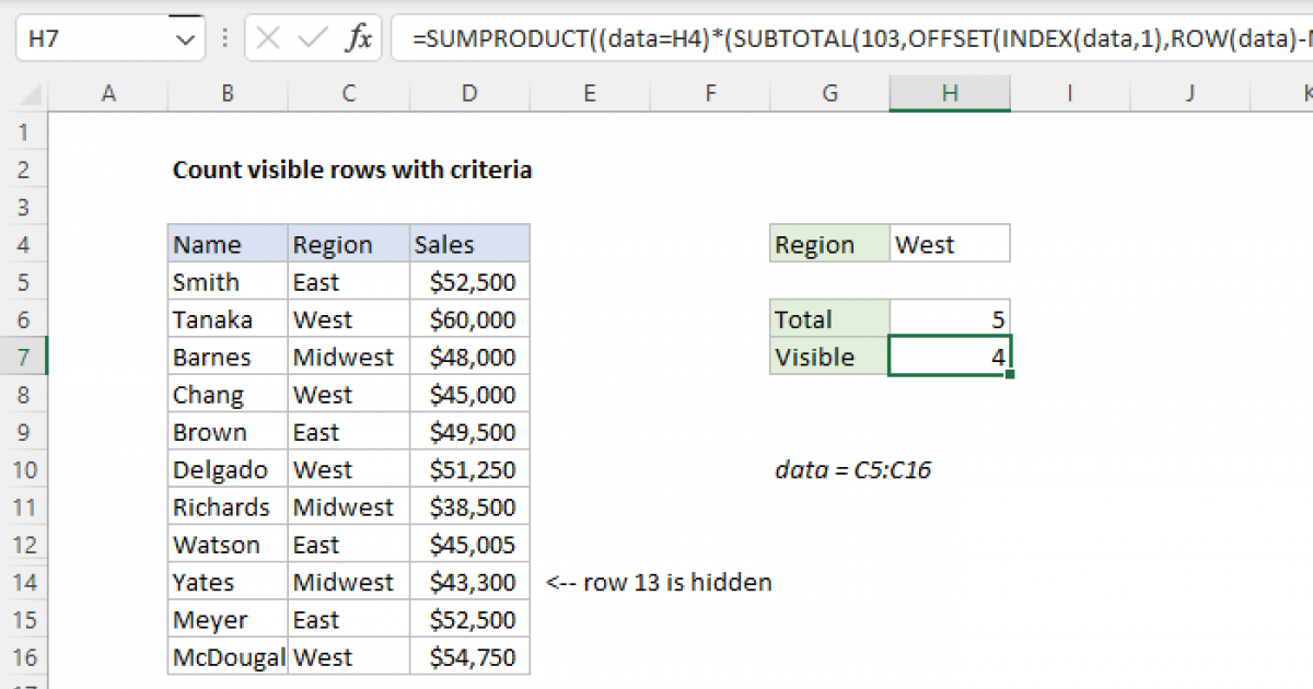
Count visible rows with criteria

To count visible rows with criteria, you can use a rather complex formula based on three main functions: SUMPRODUCT, SUBTOTAL, and OFFSET. In the example shown, the formula in H7 is: =SUMPRODUCT((data=H4)*(SUBTOTAL(103,OFFSET(INDEX(data,1),ROW(data)-MIN(ROW(data)),0)))) Where data is the named...

exceljet.net

But I think I'd need an offset inside an offset... I honestly have no idea and maybe this is down the wrong path.

Is anyone aware of a way to make this work?

I can't use VBA code in this approach because it needs to be something that can be applied quickly to any workbook and my users will not be able to do that with code.

If I need to provide any additional details or anything, let me know. I appreciate anyone taking the time to look at this.

Thank you!
Jon

 

[jasonb75]

If your example is an accurate representation of your real data then this should do it. Note that I've moved the data down to start in row 2, as you're filtering I assume that you will have headers in row 1.

Book1
	E
2	1
3	1
4	2
5	3
6	4
7	4
Sheet5

Cells with Conditional Formatting
Cell	Condition		Cell Format	Stop If True
E2:E7	Expression	=E2>MAX(SUBTOTAL(109,OFFSET(E$1,ROW(E$2:E2)-ROW(E$2),)))	text	NO

Book1
	E
2	1
3	1
4	2
7	4
Sheet5

Cells with Conditional Formatting
Cell	Condition		Cell Format	Stop If True
E2:E7	Expression	=E2>MAX(SUBTOTAL(109,OFFSET(E$1,ROW(E$2:E2)-ROW(E$2),)))	text	NO

 

[JonXL]

Thank you so much for the quick response!

If your example is an accurate representation of your real data then this should do it.

If by representative you mean all numeric, unfortunately it is not. I attempted to apply your solution to my example and it worked, but applying it to my actual data did not produce the correct results.

It must be related to the data type because when I change each 4 in my example to 4a, they are all highlighted.

Do you know what changes to your formula would be needed to get it to work with text data?

Thank you.

 

[JonXL]

I think I got it ... I played around with the formula a little and I have the following working using a combination of your solution and the info at the link in my OP:

=SUMPRODUCT(($E$1:E1=E1)*SUBTOTAL(103,OFFSET(E$1,ROW($E$1:E1)-ROW(E$1),)))=1

This works regardless of the data type in the cells. It technically doesn't meet the requirement I specified in the OP of highlighting each time the value changes, but that was a little misworded because it really just needs to highlight each distinct element once. So this does that. I also like this one because my users can apply it directly to all of column E without having to select a range of cells. I think the biggest thing I was having trouble with was getting the dynamic range established in the SUBTOTAL() function and your formula held the key to making that piece work.

I appreciate your guidance. I could not have gotten this without it! Tomorrow I will put this in my production file and see how it performs on 300,000 rows.

Thank you,
Jon

 

[jasonb75]

Tomorrow I will put this in my production file and see how it performs on 300,000 rows.

Ouch! I'm going to guess very slowly with that many rows. Thinking of other ways that might work,

Is the data sorted in a way that with the filters cleared all identical values will be in consecutive rows?

Is a helper column permissable?

 

[JonXL]

Ouch! I'm going to guess very slowly with that many rows.

It wasn't too bad. But it also turned out I only had 30,000 rows and not 300,000. I can't filter by color because the conditional formatting needs more time to calculate than the filter takes to apply so it misses most of the results.

Is the data sorted in a way that with the filters cleared all identical values will be in consecutive rows?

It is sorted, yes.

Is a helper column permissable?

I think that would be more work for users to set it up than what they'd save in performance. However... I already have a helper column in the worksheet for another purpose. The column is =G2-F2 filled down and users then filter out any that are zero. I wonder if I could reuse that column to create both a unique value to exclude for filtering and then another value for this formatting... maybe something like... =IF(G2-F2<=0,"X",IF(special formula for formatting,"Y","Z")) and then having users filter out the Xs and Zs (because at that point they wouldn't even need to keep them and could just filter them out). But I'm wondering if it would still need that volatile function that would calculate so slowly... Something I might look into, nonetheless.

 

[jasonb75]

I can't filter by color because the conditional formatting needs more time to calculate than the filter takes to apply so it misses most of the results.

I think you will find that you can only filter by colour on regular formatting, if you can filter on conditional formatting then it would be based on the state of the formats prior to the filter being applied.

But I'm wondering if it would still need that volatile function that would calculate so slowly.

Conditional formatting is a volatile function regardless of how it is done, the only thing that you can do is improve efficiency. This is the sort of thing I had in mind.
The conditional formatting formula could be shortened to just =COUNTIF(F$1:F1,F2)=0 but testing for a blank first means that the countif is not processed on the hidden rows, which makes it more efficient.

Book1
	E	F
1	List	Helper
2	a	a
3	a	a
4	a	a
5	b	b
6	c	c
7	c	c
8	c	c
Sheet9

Cells with Conditional Formatting
Cell	Condition		Cell Format	Stop If True
E2:E8	Expression	=IF(F2<>"",COUNTIF(F$1:F1,F2)=0)	text	NO

Book1
	E	F
1	List	Helper
2	a	a
3	a	a
4	a	a
5	b	b
8	c	c
Sheet9

Cells with Conditional Formatting
Cell	Condition		Cell Format	Stop If True
E2:E8	Expression	=IF(F2<>"",COUNTIF(F$1:F1,F2)=0)	text	NO