Conditional formatting | icon sets | relative reference formula

maximillianrg

Board Regular
Joined
Aug 7, 2014
Messages
74
Office Version
  1. 2016
Platform
  1. Windows
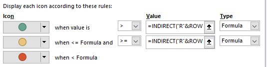
In cell A1 I have the number 100 and in cell B1 I have the Green, Yellow, Red icon set so that:

- if the value of cell B1 is greater than A1 the dot is green
- if the value of cell B1 is equal to A1 the dot is yellow
- if the value of cell B1 is less than A1 the dot is red

Applies to = $B$1 and Values of both > and >= is =$A$1

I need to apply this to over 400 rows but cant figure out how to do it as excel barks at me when I try and remove the $ and says "you cannot use relative references in conditional formatting for color scales, data bars, and icon sets" and format painter does not work either. I really don't want to set this up 400 times in a row - Help?
 

Excel Facts

Enter current date or time
Ctrl+: enters current time. Ctrl+; enters current date. Use Ctrl+: Ctrl+; Enter for current date & time.
Well, ya can't do that. When Microsoft fixes this deficiency there will be a national holiday declared.

But don't hold your breath. If you don't mind having the Icon Sets appear in the cell beside your target cell, try this. And when I say 'appear' I mean 'appear to appear' because the Icon Sets cannot be adapted.

In A1 put 100, which is our control value. In B1 through B3 put 120, 100, and 80 respectively (and so on for 400 rows). In C1 through C3, paste =UNCIDOE(11044) and then colour the font some shade of red. Select cells C1 through C3. Create two new CondFrmt rules: 1) =B1=A1 and choose some shade of yellow for the font; 2) =B1>A1 and choose some shade of green for the font.<strike></strike>


This thread (https://www.mrexcel.com/forum/excel...c-lights-unrimmed-conditional-formatting.html) tells me that the RGB values for the Excels Traffic Lights icons are as follows:
Green: 104,164,144
Amber: 234,194,130
Red: 192,80,77

This reference has all the Unicode characters you could ever wish to look at; this is where I got character 11044, which is a big ole dot. http://www.grogllc.com/unicodetable.html#<strike></strike><strike></strike><strike></strike><strike></strike><strike></strike><strike></strike><strike></strike><strike></strike><strike>
</strike>
 
Last edited:
Upvote 0
not sure if this is still an issue, but though tricky with the format painter, you can use the INDIRECT function to get around the relative reference issue...
for the example above... if you're comparing B1 to A1 and want to paste it down... the "formula" field it would be:
=INDIRECT("R"&ROW()&"C" & COLUMN()-1, FALSE)

The trick is, you can't just use the format painter to apply to all 400 rows at once.
You will need to first manually put the formula in say 10 rows.. then do format painter in increments of 10

In my issue, I was comparing values in Column D to Column J, so my formula was:
=INDIRECT("R"&ROW()&"C" & COLUMN()+6, FALSE)

basically.. your +/- number is adjusted based on how many columns to the right (+) or left(-) your comparison number is located
same can be applied to the "row" portion of the formula if needed for vertical comparisons

hope this helps!
 

Attachments

  • excelsnip.PNG
    excelsnip.PNG
    7.2 KB · Views: 117
Upvote 0

Forum statistics

Threads
1,214,920
Messages
6,122,279
Members
449,075
Latest member
staticfluids

We've detected that you are using an adblocker.

We have a great community of people providing Excel help here, but the hosting costs are enormous. You can help keep this site running by allowing ads on MrExcel.com.
Allow Ads at MrExcel

Which adblocker are you using?

Disable AdBlock

Follow these easy steps to disable AdBlock

1)Click on the icon in the browser’s toolbar.
2)Click on the icon in the browser’s toolbar.
2)Click on the "Pause on this site" option.
Go back

Disable AdBlock Plus

Follow these easy steps to disable AdBlock Plus

1)Click on the icon in the browser’s toolbar.
2)Click on the toggle to disable it for "mrexcel.com".
Go back

Disable uBlock Origin

Follow these easy steps to disable uBlock Origin

1)Click on the icon in the browser’s toolbar.
2)Click on the "Power" button.
3)Click on the "Refresh" button.
Go back

Disable uBlock

Follow these easy steps to disable uBlock

1)Click on the icon in the browser’s toolbar.
2)Click on the "Power" button.
3)Click on the "Refresh" button.
Go back
Back
Top