AMANDAJELLIOTT
New Member
- Joined
- Jul 20, 2021
- Messages
- 6
- Office Version
- 2013
- Platform
- Windows
Hi!
This wonderful forum helped me out a while back with a work project I just could not figure out. I am back again with a similar work project that is throwing me for a loop and was hoping you guys could help me learn where I am going wrong. I'm not understanding something about my formulas, and I want to learn!
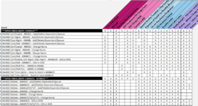
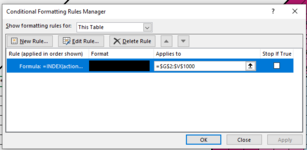
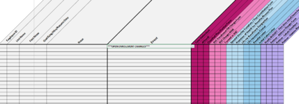
I have a workbook that has been created for a department within my company. This workbook has an actions table tab that contains list of events and each action that needs to be taken for each event. The tasks that do not need to be completed have an "X" in the cell, the tasks that do need to be completed have a blank cell. Under the MASTER tab, I have created a drop down list for the user to select an event. Once they have made their selection, I have inserted a conditional formatting expression to fill in each cell that had an "X" on my actions table tab as black. This way, the user only sees what actions they need to complete based on the event they have chosen.
BUT, this is not working and I dont know why. I have looked at this for so long my eyes are crossing . Can someone please help?
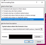
The forumla I have inserted in conditional formatting is: =INDEX(actions_Table!C$5:R$29,MATCH($F2,actions_Table!$B$5:$B$29,0))="X"
Thank you so much for your assistance!
This wonderful forum helped me out a while back with a work project I just could not figure out. I am back again with a similar work project that is throwing me for a loop and was hoping you guys could help me learn where I am going wrong. I'm not understanding something about my formulas, and I want to learn!
I have a workbook that has been created for a department within my company. This workbook has an actions table tab that contains list of events and each action that needs to be taken for each event. The tasks that do not need to be completed have an "X" in the cell, the tasks that do need to be completed have a blank cell. Under the MASTER tab, I have created a drop down list for the user to select an event. Once they have made their selection, I have inserted a conditional formatting expression to fill in each cell that had an "X" on my actions table tab as black. This way, the user only sees what actions they need to complete based on the event they have chosen.
BUT, this is not working and I dont know why. I have looked at this for so long my eyes are crossing
. Can someone please help? The forumla I have inserted in conditional formatting is: =INDEX(actions_Table!C$5:R$29,MATCH($F2,actions_Table!$B$5:$B$29,0))="X"
Thank you so much for your assistance!