Conditional Formatting limiting it to items listed in name range.

[Livin404]

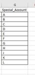
Good evening, I'm confident this should be straight forward, but nonetheless I find myself stuck. I have a formula I'm currently using =SUMPRODUCT(--ISNUMBER(SEARCH(Special_Account,$G2))). The special account is in the image. It is the letter preceded by a space. I want it limited to just that-(two characters- the space then the letter. If I get something like H1952035 it will not highlight because the letter H is in the name range. I'm looking for one space and one letter found in the name range and nothing else.

As always much appreciated.

 

[JoeMo]

Try this CF formula applied to G2 and down to whatever you want:
=AND(LEN($G2)=2, COUNTIF(Special_Account,$G2)>0)

 

[Livin404]

Works perfect thank you!

 

[Peter_SSs]

Whilst I agree that will work fine, either of these much simpler CF formulas should also do the job.

=COUNTIF(Special_Account,G2)
=MATCH(G2,Special_Account,0)

 

[Livin404]

Thank you, since you’re here I’m trying to find the formula to highlight blank cells. I know the obvious way, but what I am using is a template to let the user know if there are errors and one of those is for blank cells. The problem is the number of rows are variable. So I’m looking for the conditional format formula that will locate the last row in a Column and highlight only blank cells from row 1 down to the last filled row. As it stands now the whole sheet is yellow and hard to look at. This would be from Column A to H and theN J to V.
Thank you.

 

[Peter_SSs]

Try applying CF like this to all cells down as far as you might ever need. In this example I have applied to row 100. If you apply to more or less rows then also adjust the range in the CF formula.

20 10 11.xlsm
	A
1	x
2
3	x
4	x
5	x
6
7	x
8
9
10
11
12
13	x
14	x
15
16	x
17
18
19
20
CF

Cells with Conditional Formatting
Cell	Condition		Cell Format	Stop If True
A1:A100	Expression	=AND(A1="",COUNTA(A1:A$100))	text	NO