CONDITIONAL FORMATTING NEEDED TO SKIP EMPTY ROWS UNTIL THE NEXT SECTION OF DATA

[JuicyMusic]

Hello, I am quickly learning how to set up more complex conditional formatting by coming here and reading other posts and solutions. I am so excited
to see how to do adjust or write this CF that I now need..... but this one is beyond me at this point.........Thank you Mr.Excel!!

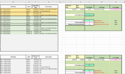
I have 2 CF's on one continuous spreadsheet (no blank rows) that alternates between two colors based on the job number change in column E.
but now I have had to revise the spreadsheet and now need the CF to skip blank rows - and then to start formatting again at the next section of data (going down) - at the first occurrence of either of these three texts (they will never be any other text):

JSA
TAIL GATE MEETING
PANDEMIC JOB HAZARD ANALYSIS

1) The header row of the 1st section of data may vary. Please let me know if it should be fixed. If it should be fixed then the header of the 1st section will always start on row 13.
2) The CF should encompass columns D thru G.
3) The trigger for the next color is the Job Number in column E
4) The number of sections of data will vary
4) The number of rows per section of data will vary. From 13 rows at the minimum to 75 rows. In case you need to know (but I don't think so )
5) The header names of the 4 columns will not change. Same for each section. See snippet uploaded.

I'm asking for assistance so that I don't have to set the same CF over and over again for every section. Here is a snapshot of my spreadsheet and the CF. Thank you!!

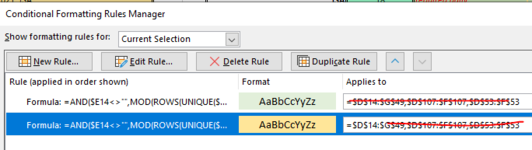
CF 1:

=AND($E14<>"",MOD(ROWS(UNIQUE($E$14:$E14)),2)=0)

CF 2:

=AND($E14<>"",MOD(ROWS(UNIQUE($E$14:$E14)),2)=1)

 

[Marcelo Branco]

Is this what you want?
As I'm using XL2010 I don't have the UNIQUE function, so the formulas are more complex, but they should also work in 365.

11082021 Testes.xlsx
	D	E	F	G
13	Full Name	Job #	Date	Form Name
14	Name1	A	01/01/2021	Pandemic
15	Name1	A	02/01/2021	Tail
16	Name1	B	03/01/2021	JSA
17	Name1	B	04/01/2021	Pandemic
18	Name1	C	05/01/2021	JSA
19	Name1	C	06/01/2021	Tail
20	Name1	D	07/01/2021	Pandemic
21	Name1	D	08/01/2021	JSA
22	Name1	E	09/01/2021	Tail
23	Name1	F	10/01/2021	Pandemic
24	Name1	F	11/01/2021	JSA
25	Name1	F	12/01/2021	Tail
26	Name1	G	13/01/2021	JSA
27	Name1	G	14/01/2021	Tail
28
29
30
31
32
33
34
35	Full Name	Job #	Date	Form Name
36	Name2	H	15/01/2021	JSA
37	Name2	I	16/01/2021	Pandemic
38	Name2	I	17/01/2021	Tail
39	Name2	J	18/01/2021	Pandemic
40	Name2	K	19/01/2021	Tail
41	Name2	K	20/01/2021	JSA
42	Name2	L	21/01/2021	Pandemic
43
44
45
Plan8

Cells with Conditional Formatting
Cell	Condition		Cell Format	Stop If True
D14:G105	Expression	=E($E14<>"";$E14<>"Job #";MOD(SOMA(SE(FREQÜÊNCIA(SE($E$14:$E14<>"";SE($E$14:$E14<>"Job #";CORRESP($E$14:$E14;$E$14:$E14;0)));LIN($E$14:$E14)-LIN($E$14)+1);1));2)=0)	text	NO
D14:G105	Expression	=E($E14<>"";$E14<>"Job #";MOD(SOMA(SE(FREQÜÊNCIA(SE($E$14:$E14<>"";SE($E$14:$E14<>"Job #";CORRESP($E$14:$E14;$E$14:$E14;0)));LIN($E$14:$E14)-LIN($E$14)+1);1));2)=1)	text	NO

Translating the CF formulas to English
=AND($E14<>"",$E14<>"Job #",MOD(SUM(IF(FREQUENCY(IF($E$14:$E14<>"",IF($E$14:$E14<>"Job #",MATCH($E$14:$E14,$E$14:$E14,0))),ROW($E$14:$E14)-ROW($E$14)+1),1)),2)=1)
Fill --> Light orange

=AND($E14<>"",$E14<>"Job #",MOD(SUM(IF(FREQUENCY(IF($E$14:$E14<>"",IF($E$14:$E14<>"Job #",MATCH($E$14:$E14,$E$14:$E14,0))),ROW($E$14:$E14)-ROW($E$14)+1),1)),2)=0)
Fill --> Light green

Hope this helps

M.

 

[Fluff]

Another option for 365

+Fluff 1.xlsm
	D	E	F	G
13	Full Name	Job #	Date	Form Name
14	Name1	A	01/01/2021	Pandemic
15	Name1	A	02/01/2021	Tail
16	Name1	B	03/01/2021	JSA
17	Name1	B	04/01/2021	Pandemic
18	Name1	C	05/01/2021	JSA
19	Name1	C	06/01/2021	Tail
20	Name1	D	07/01/2021	Pandemic
21	Name1	D	08/01/2021	JSA
22	Name1	E	09/01/2021	Tail
23	Name1	F	10/01/2021	Pandemic
24	Name1	F	11/01/2021	JSA
25	Name1	F	12/01/2021	Tail
26	Name1	G	13/01/2021	JSA
27	Name1	G	14/01/2021	Tail
28
29
30
31
32
33
34
35	Full Name	Job #	Date	Form Name
36	Name2	H	15/01/2021	JSA
37	Name2	I	16/01/2021	Pandemic
38	Name2	I	17/01/2021	Tail
39	Name2	J	18/01/2021	Pandemic
40	Name2	K	19/01/2021	Tail
41	Name2	K	20/01/2021	JSA
42	Name2	L	21/01/2021	Pandemic
43
44
Main

Cells with Conditional Formatting
Cell	Condition		Cell Format	Stop If True
D14:G100	Expression	=AND($E14<>"",$E13<>"",MOD(COUNTA(UNIQUE($E$13:$E14)),2)=0)	text	NO
D14:G100	Expression	=AND($E14<>"",$E13<>"",MOD(COUNTA(UNIQUE($E$13:$E14)),2)<>0)	text	NO

 

[Marcelo Branco]

Fluff,

Just out of curiosity, would this work in 365?
=AND($E14<>"",$E13<>"",MOD(ROWS(UNIQUE(FILTER($E$13:$E14,$E$13:$E14"<>"))),2)=0)

M.

 

[Fluff]

With a minor tweak, yes

+Fluff 1.xlsm
	D	E	F	G
13	Full Name	Job #	Date	Form Name
14	Name1	A	01/01/2021	Pandemic
15	Name1	A	02/01/2021	Tail
16	Name1	B	03/01/2021	JSA
17	Name1	B	04/01/2021	Pandemic
18	Name1	C	05/01/2021	JSA
19	Name1	C	06/01/2021	Tail
20	Name1	D	07/01/2021	Pandemic
21	Name1	D	08/01/2021	JSA
22	Name1	E	09/01/2021	Tail
23	Name1	F	10/01/2021	Pandemic
24	Name1	F	11/01/2021	JSA
25	Name1	F	12/01/2021	Tail
26	Name1	G	13/01/2021	JSA
27	Name1	G	14/01/2021	Tail
28
29
30
31
32
33
34
35	Full Name	Job #	Date	Form Name
36	Name2	H	15/01/2021	JSA
37	Name2	I	16/01/2021	Pandemic
38	Name2	I	17/01/2021	Tail
39	Name2	J	18/01/2021	Pandemic
40	Name2	K	19/01/2021	Tail
41	Name2	K	20/01/2021	JSA
42	Name2	L	21/01/2021	Pandemic
43
44
45
46
Main

Cells with Conditional Formatting
Cell	Condition		Cell Format	Stop If True
G14:G46	Expression	=AND($E14<>"",$E13<>"",MOD(ROWS(UNIQUE(FILTER($E$13:$E14,$E$13:$E14<>""))),2)<>0)	text	NO
G14:G46	Expression	=AND($E14<>"",$E13<>"",MOD(ROWS(UNIQUE(FILTER($E$13:$E14,$E$13:$E14<>""))),2)=0)	text	NO
D14:G100	Expression	=AND($E14<>"",$E13<>"",MOD(COUNTA(UNIQUE($E$13:$E14)),2)=0)	text	NO
D14:G100	Expression	=AND($E14<>"",$E13<>"",MOD(COUNTA(UNIQUE($E$13:$E14)),2)<>0)	text	NO

 

[Marcelo Branco]

With a minor tweak, yes

Thank you. I'm trying to learn how to use the new functions even do not having (yet) 365

M.

 

[JuicyMusic]

Hello Marcelo, I did use your first set and it freaked the CF box out....I had to close the spreadsheet. It looked like it colored the header of the next section instead of the 1st row below the header row of each new section.

Thank you so so much for your input. I actually printed out this whole post because I want to breakdown each that you guys sent me. All of them.

Fluff, Your formula worked great. Thank you again for solving. If I can talk the formula out then I can write these.

 

[Fluff]

Glad we could help & thanks for the feedback.