Conditional Formatting not giving true results

[The Shadowman]

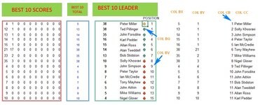
Column BQ =INDEX($C:$C,AGGREGATE(15,6,ROW($C$31:$C$45)/($BX$31:$BX$45=LARGE($BX$31:$BX$45,ROWS(CC$26:CC26))),COUNTIF(BN$31:BN31,BN31)))
Column BV =RANK(LARGE($BN$31:$BN$45,ROWS($BV31:$BV$31)),$BN$31:$BN$45)
Column BX =SUM(D31:AG31)
Column BY =BX31-INDEX($D31:$AG31,AGGREGATE(14,6,COLUMN($D$31:$AG$31)-COLUMN($C$31)/($D$32:$AG$45>0),1))
Column CB =RANK(LARGE($BY$31:$BY$45,ROWS($CB$31:$CB31)),$BY$31:$BY$45)
Column CC =INDEX($C:$C,AGGREGATE(15,6,ROW($C$31:$C$45)/($BY$31:$BY$45=LARGE($BY$31:$BY$45,ROWS(CB$31:CB31))),COUNTIF(CB$31:CB31,CB31)))

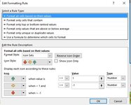
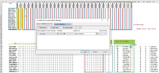
Hi I thought all was well with this project, but I have discovered that the conditional formatting is not working correctly. It's not far out, but something is wrong giving the wrong result. The formulas above are, as far as I know, the one s that control it, but I am not sure.
I have uploaded a couple of pictures that will, I hope, help you see what's going wrong.
It's driving me mad so any help you can offer will be greatly appreciated.
Thanks
Robert

 

[6StringJazzer]

What is the Applies To range for the rule you showed in your second screen shot?

Do you have four hidden columns between the two blue arrows in your first screen shot?

The rule applies to the cell containing the data but your first screen shot does not show us what the data is that the rule is using. What is the data in column BQ for Pete, John, Ted, Karl, etc."

That is, we can't tell why you think it's not working.

 

[The Shadowman]

What is the Applies To range for the rule you showed in your second screen shot?

Do you have four hidden columns between the two blue arrows in your first screen shot?

The rule applies to the cell containing the data but your first screen shot does not show us what the data is that the rule is using. What is the data in column BQ for Pete, John, Ted, Karl, etc."

That is, we can't tell why you think it's not working.

Thanks for replying so quickly.

The conditional formatting applies to =$BU$31:$BU$45. There are 4 hidden columns, they are BX, BY, CB and CC. BX refers to GRAND TOTAL this week =SUM(D31:AG31),
BY is GRAND TOTAL last week =BX31-INDEX($D31:$AG31,AGGREGATE(14,6,COLUMN($D$31:$AG$31)-COLUMN($C$31)/($D$32:$AG$45>0),1)),
CB should be POSITION THIS WEEK, but is it working?=RANK(LARGE($BY$31:$BY$45,ROWS($CB$31:$CB31)),$BY$31:$BY$45)
CC is LEADERBOARD LAST WEEK =INDEX($C:$C,AGGREGATE(15,6,ROW($C$31:$C$45)/($BY$31:$BY$45=LARGE($BY$31:$BY$45,ROWS(CB$31:CB31))),COUNTIF(CB$31:CB31,CB31)))
I hope you can understand the above

Thanks

Robert

 

[6StringJazzer]

That is different that what you provided in your first post. In your first post you said this data was in BQ.

Nevertheless, the icon conditional formatting applies to the data in the cell you are formatting, and you are not showing that data. You did not answer my third question, which is actually the most important. What is the actual data in the cells BU31:BU45? You can copy the cells and paste them right into a post (better than screen shots).

 

[The Shadowman]

BU31:45 =MATCH($BQ31,$CC$31:$CC$45,0)-(ROW()-ROW($CX$30)) refers to leaderboard this week. I don't know why $CX$30 is in the formula. it was part of a suggested formula from my original post. The leaderboard gets it's info from =INDEX($C:$C,AGGREGATE(15,6,ROW($C$31:$C$45)/($BX$31:$BX$45=LARGE($BX$31:$BX$45,ROWS(CC$26:CC26))),COUNTIF(BN$31:BN31,BN31))).
You have most likely gathered that I am fairly new to Excel and finding these complicated formulas a little difficult to get my head round so any help is greatly appreciated. Have I answered your question correctly? If not please let me know.

Thanks
Robert

 

[6StringJazzer]

We are going in circles. The formula doesn't matter. I need to see the values, because the values are what are used by the conditional formatting rule.

Your cells in BU are showing the icons, but not the values. You are saying you are getting the wrong results, but if you don't see the values, how do you know the results are wrong? I am expecting to see something like this in your sheet. I set this using the same rule as you:

 

[The Shadowman]

I couldn't get the icons to show so I have attached a screenshot. I hope that is OK

 

[6StringJazzer]

Your conditional formatting rule that you showed in your first post says:

Value is	Icon
>= 1	Green Up Arrow
< 1 and >= -1	Yellow Right Arrow
< -1	Red Down Arrow

This is exactly what your screen shot in post #7 shows is happening.

the conditional formatting is not working correctly

What are you expecting to happen instead?

 

[The Shadowman]

One example is: place number one, when relegated to, for example, second place gains a yellow right arrow instead of a red down arrow. I can not work why this happens.

Thanks again

 

[6StringJazzer]

I don't know what that means relative to the data you showed. What does "place number one relegated to second place" mean? There is nothing in your screenshot that suggest what is a "place." Remember that you built this file and you know what everything means but we have never seen it before and have no idea what you are doing. The conditional formatting just works on whatever numbers you have in the cells (-2, 1, 5, 7....) and it is working correctly. I suspect that you have some other issue that is putting the wrong number into those cells. But I don't know what those numbers are supposed to mean.