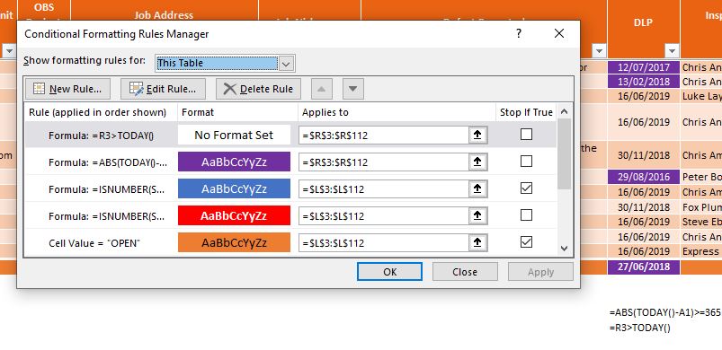
Conditional Formatting on Cell that is outside the 365 days warranty end date

[gplans]

I am trying to set some conditional formatting on cell that are outside the 365 days warranty end date that is entered into the cell.

[TABLE="width: 101"]
<colgroup><col></colgroup><tbody>[TR]
[TD][TABLE="width: 101"]
<colgroup><col></colgroup><tbody>[TR]
[TD][TABLE="width: 296"]
<colgroup><col><col></colgroup><tbody>[TR]
[TD]19/07/2019[/TD]
[TD]Within warranty[/TD]
[/TR]
[TR]
[TD]30/11/2018[/TD]
[TD]Highlighted cell warranty ended[/TD]
[/TR]
[TR]
[TD]16/06/2019[/TD]
[TD]Within warranty[/TD]
[/TR]
[TR]
[TD]19/07/2019[/TD]
[TD]Within warranty[/TD]
[/TR]
</tbody>[/TABLE]
[/TD]
[/TR]
</tbody>[/TABLE]
[/TD]
[/TR]
</tbody>[/TABLE]

Cant seem to find anything that matches my criteria. Any help thanks.

 

[sandy666]

try =ABS(TODAY()-G1)>=365

30/11/2018 this date does not meet your condition, try 26/06/2018 instead

 

[gplans]

try =ABS(TODAY()-G1)>=365

30/11/2018 this date does not meet your condition, try 26/06/2018 instead

This did not work.

It highlighted 15/02/2020 only in these dates. In this case 29/08/2016 was the last day the warranty expired and that should have been the date highlighted.

[TABLE="width: 101"]
<colgroup><col></colgroup><tbody>[TR]
[TD]29/08/2016[/TD]
[/TR]
[TR]
[TD]16/06/2019[/TD]
[/TR]
[TR]
[TD]15/02/2020[/TD]
[/TR]
[TR]
[TD]15/02/2020[/TD]
[/TR]
[TR]
[TD]15/02/2020[/TD]
[/TR]
</tbody>[/TABLE]

I found how this formula works:

For future dates, higher than today’s date, use B1-TODAY() in the logical test argument.
If the date is smaller than today’s date, use TODAY()-B1.
If you want this to work in both ways, use ABS(TODAY()-B1)

 

[sandy666]

[Table="width:, class:head"]
[tr=bgcolor:#FFFFFF][td=bgcolor:#FFFF00]

29/08/2016​

[/td][/tr]

[tr=bgcolor:#FFFFFF][td]

16/06/2019​

[/td][/tr]

[tr=bgcolor:#FFFFFF][td]

15/02/2020​

[/td][/tr]

[tr=bgcolor:#FFFFFF][td]

15/02/2020​

[/td][/tr]

[tr=bgcolor:#FFFFFF][td]

15/02/2020​

[/td][/tr]
[/table]

so it works

edit:
I just copied your dates from post above and paste into the same range. you need to resize range of Conditional Formatting and adjust G1 to your needs of course

Example CF

 

[sandy666]

future date ( 15/02/2020 ) will be highlighted if today()-15/02/2020>=365

 

[gplans]

Ok yes yours works but the formula is not working as intended.

An item has a warranty on it and it only last 1 year. The date of the warranty are from:

29/08/2015 to 29/08/2015 - This need to be highlighted
29/08/2019 to 29/08/2020 - This does not need to be highlighted
16/08/2018 to 16/08/2019 - This need to be highlighted

The date shown is the last day the warranty expires.

Thanks for helping.

 

[sandy666]

you can try this way where no color is the first then color:

 

[gplans]

I am not sure what is happening.

I did it your way on a new sheet and it works but when I try it on my sheet it does not.

 

[sandy666]

=R3>TODAY() must be on top

 

[gplans]

=R3>TODAY() must be on top

No that did not do the trick either.