Conditional Formatting with a Vlookup formula

[Rosstamon]

Hello,
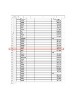
I have a spreadsheet with 36 rows of data in columns F – I, rows 2 – 36, and row 1 is the header info.
Column F has alphabetical symbols.
Column I contains numbers expressed as percentages.

I would like to be able to do the following:
If column F contains alphabetical symbol “ANDI”, highlight the entire line (F – I) grey. This could be row 18 this time, and row 22 next time and could always change. I believe this conditional formula would look like this:
=$F2="ANDI", then custom format grey and apply it to $F$2:$I$36

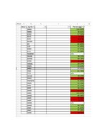
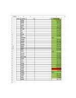
Here's where it gets tricky for me, I would like the remaining conditional formatting to do the following for column I in each row:

"if the number in column I, in each row is greater than column I of the row that contains the symbol "ANDI", then highlight the number green.

"if the number in column I, in each row is less than the number in column I of the row that contains the symbol "ANDI”, then highlight the number red.

I'm stuck and would appreciate any help. I’m dreadfully awful at VBA, so I don’t think that would work for me.

I've attached an example of what it would look like before and after conditional formatting.

Thank you

 

[jasonb75]

Assuming that "ANDI" is only found once in column F, use this for green rule, change > to < for red rule.

=$I2>SUMIF($F$2:$F$36,"ANDI",$I$2:$I$36)

 

[Rosstamon]

Assuming that "ANDI" is only found once in column F, use this for green rule, change > to < for red rule.

=$I2>SUMIF($F$2:$F$36,"ANDI",$I$2:$I$36)

I appreciate the help, it didn't work. Also, I just realized I kept using "I" where I should have been using "J", so I changed your formulas as follows, but it still didn't work:
=$J2<SUMIF($F$2:$F$36,"ANDI",$J$2:$J$36) and the custom is fill red.
=$J2>SUMIF($F$2:$F$36,"ANDI",$J$2:$J$36) and the custom fill is green.

The result is the following.

Any other ideas.
I really appreciate your help. Would love to get this working right.
Thanks again.


***EDIT***
Your formulas are exactly correct, I also needed to change "F" to "G". I apologize. I must have had it as "F - I" originally, and moved it over one column at some point. At any rate, your suggestion made it work once I got my targets corrected. Thank you so much.