Conditional Formatting with data validation list

[fatekeeper]

I am trying to create an excel file that will allow order information to be entered and then to allow for the status of each line to be tracked and also to have color coding to flag orders depending on the ship date.

I created a worksheet that uses a drop down box (pulls from a list on a different worksheet in the same workbook) so the user can select different statuses, and I applied conditional formatting to change the color of each line slightly so the users know at a glance which orders are in which status. My problem comes when trying to apply conditional formatting to cells in a column that displays the estimated ship date. I want the cell with the ship date and to turn green fill for orders shipping within the next week (7 days) to help flag them for follow-up and red fill if the date has already passed, but not to change if the status column indicates it has already shipped.
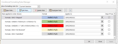
I have the conditional formatting rule for Shipped status as the first one have it marked to stop if that rule is triggered, which is working as expected. My issue is that now when any other status is selected, if there is not yet a date in the ship date field, it remains red. I would like it to stay the same color as the status would indicate UNLESS it's a date in the next 7 days (fill green) or a past date but not yet shipped (fill red) - is there a way to do this?

Enersys Order Tracker.xlsx
	A	B	C	D	E	F	G	H
1	Date Submitted	Customer	PO#	MATERIAL	Quote#	ESD	Notes	Status
2	11/1/2021		1234	SAMPLE1	QN2021-08	12/30/2021		Shipped
3	12/20/2021		5678	SAMPLE2	QN2022-02	12/31/2021		OA Received
4	1/3/2022		2468	SAMPLE3	QN2022-01			Submitted
5
Open Orders

Cells with Conditional Formatting
Cell	Condition		Cell Format	Stop If True
F3:F5	Expression	=$H3="Shipped"	text	YES
F3:F5	Expression	=AND(F3>TODAY(),F3<=(TODAY()+7))	text	NO
F3:F5	Expression	=$F3=(TODAY()-$F$2)>=1	text	NO
F3:F5	Expression	=$H3="OA Received"	text	NO
F3:F5	Expression	=$H3="Submitted"	text	NO
A2:G2	Expression	=$H2="Shipped"	text	YES
F2	Expression	=AND(F2>TODAY(),F2<=(TODAY()+7))	text	NO
H3:H2000	Cell Value	=Lists!$A$4	text	NO
H3:H2000	Cell Value	=Lists!$A$3	text	NO
H3:H2000	Cell Value	=Lists!$A$2	text	NO
A6:G2050,A5:E5,G5	Expression	=$H5="Shipped"	text	NO
A6:G2050,A5:E5,G5	Expression	=$H5="OA Received"	text	NO
A6:G2050,A5:E5,G5	Expression	=$H5="Submitted"	text	NO
A3:E4,G3:G4	Expression	=$H3="Shipped"	text	NO
A3:E4,G3:G4	Expression	=$H3="OA Received"	text	NO
A3:E4,G3:G4	Expression	=$H3="Submitted"	text	NO
F2	Expression	=$F2=(TODAY()-$F$2)>=1	text	NO
A2:G2	Expression	=$H2="OA Received"	text	NO
A2:G2	Expression	=$H2="Submitted"	text	NO
H2	Cell Value	=Lists!$A$4	text	NO
H2	Cell Value	=Lists!$A$3	text	NO
H2	Cell Value	=Lists!$A$2	text	NO

Cells with Data Validation
Cell	Allow	Criteria
H2:H4	List	=Lists!$A:$A
H5	List	=Lists!$A:$A

 

[Toadstool]

Hi Fatekeeper,

Try

=AND($F3<>"",($F3=(TODAY()-$F$2)>=1))

 

[fatekeeper]

Thank you! It worked perfectly!

 

[Toadstool]

You're welcome. Glad to help.

 

[fatekeeper]

Hi again! Adding this as a comment instead as a new thread since it is related and I think the previous history might be useful. Now that the user is inputting data, some of the rules aren't working.
Basically, if the status from the drop down list is "Shipped", the cells behave as desired, and if the estimated ship date falls within 7 days from today the cells also behave as desired (fill green in date column).
But for any other status selected and regardless of the date entered in the date column (except for those within 7 days in the future from today), all cells in the date column that have a date entered are filling red, which should only happen for dates that occur prior to today. The rule appears to be the same as previously advised to try, and it worked when I tried it originally but now that the user is manipulating the data I cannot for the life of me figure out why it's not working. I've tried a bunch of different changes but none give the desired result. I've attached a screenshot for the rules in place when cell F3 is selected - hopefully a more experienced set of eyes can see what I'm obviously overlooking and explain what I'm doing wrong? Thank you.

 

[Toadstool]

Please supply more data using XL2BB.
Your red CF is always based on cell $F$2 but without seeing more sample data I'm not sure if it should be relative.

 

[fatekeeper]

SAMPLE_TRACKER.xlsx
	A	B	C	D	E	F	G	H
1	Date Submitted	Customer	PO#	MATERIAL OR PROJECT	Quote#	ESD	Notes	Status
2	10/1/2021	129554	2100574012	BATTERY & RACK		4/1/2022		OA Received
3	10/16/2021	100156	289206	BATTERY & RACK		4/1/2022		OA Received
4	11/4/2021	100113	9742142	BATTERY		2/11/2022		OA Received
5	11/19/2021	100099	9782664	BATTERY		6/3/2022		OA Received
6	11/26/2021	126237	4500311290	BATTERY		12/10/2021		Shipped
7	12/2/2021	157666	105144	TP2		3/18/2022		OA Received
8	11/23/2021	157666	105237	TP5D		12/13/2022		OA Received
9	11/23/2021	157666	105219	TP5B		12/13/2022		OA Received
10	11/12/2021	157666	104962	TP1		3/11/2022		OA Received
11	11/23/2021	157666	105153	TP5A		12/13/2022		OA Received
12	11/23/2021	157666	105228	TP5C		12/13/2022		OA Received
13	11/19/2021	157666	105091	TP3		12/30/2022		OA Received
14	12/2/2021	100111	9808681	BATTERY		6/17/2022		OA Received
15	12/1/2021	100111	9803559	BATTERY		3/10/2022		OA Received
16	11/19/2021	112329	4500728994	BATTERY		2/25/2022		OA Received
17	12/6/2021	100100	9799030	RACK		1/14/2022		OA Received
18	11/26/2021	112329	4500730746	BATTERY		1/31/2022		OA Received
19	12/10/2021	100100	9799065	RACK		1/26/2022		OA Received
20	12/11/2021	100156	290689	BATTERY & charger		6/24/2022		OA Received
21	12/17/2021	100100	9834933	RACK		2/9/2022		OA Received
22	12/22/2021	129554	2100591760	RACK		3/4/2022		OA Received
23	12/22/2021	129548	2100589581	RACK		2/18/2022		OA Received
24	12/15/2021	100100	9823941	BATTERY		3/25/2022		OA Received
25	12/23/2021	100111	9844665	BATTERY		1/27/2022		OA Received
26	12/20/2021	184985	44279-704091205	BATTERY, RACK, & CHARGER		4/26/2022		OA Received
27	12/23/2021	100099	9853564	RACK		2/16/2022		OA Received
28	12/16/2021	100100	9828307	RACK		2/9/2022		OA Received
STATUS TRACKER

Cells with Conditional Formatting
Cell	Condition		Cell Format	Stop If True
H3:H28	Expression	=$H3="Shipped"	text	NO
H3:H28	Expression	=$H3="OA Received"	text	NO
H3:H28	Expression	=$H3="Submitted"	text	NO
H2	Expression	=$H2="Shipped"	text	NO
H2	Expression	=$H2="OA Received"	text	NO
H2	Expression	=$H2="Submitted"	text	NO
F2:F2021	Expression	=AND(F2>TODAY(),F2<=(TODAY()+7))	text	NO
F2:F2021	Expression	=AND(F2>TODAY(),F2<=(TODAY()-7))	text	NO
F2:F2021	Expression	=$H2="Shipped"	text	YES
A4:C4,G4,B14:B15,B25	Expression	=$H4="Shipped"	text	NO
A4:C4,G4,B14:B15,B25	Expression	=$H4="OA Received"	text	NO
A4:C4,G4,B14:B15,B25	Expression	=$H4="Submitted"	text	NO
G2:G3,D4:E4,A14:A15,C14:G14,A26:G2049,A25,A2:E3,A5:G13,C15,A16:C16,D15:G16,A17:G24,C25:G25	Expression	=$H2="Shipped"	text	NO
G2:G3,D4:E4,A14:A15,C14:G14,A26:G2049,A25,A2:E3,A5:G13,C15,A16:C16,D15:G16,A17:G24,C25:G25	Expression	=$H2="OA Received"	text	NO
G2:G3,D4:E4,A14:A15,C14:G14,A26:G2049,A25,A2:E3,A5:G13,C15,A16:C16,D15:G16,A17:G24,C25:G25	Expression	=$H2="Submitted"	text	NO
F2:F2021	Expression	=$H2="OA Received"	text	NO
F2:F2021	Expression	=$H2="Submitted"	text	NO

Cells with Data Validation
Cell	Allow	Criteria
H2:H28	List	=Lists!$A$1:$A$4

 

[fatekeeper]

I'm trying to have the color of the cell in column F change dependent mostly on the date but also on the status:
If status in column H for the row is "Shipped", then the color of the cell in column F of that row should be blue like the rest of the row (as seen on Line 6).
If the date in column F is within seven days of today's date, I want it to fill green (as seen in row 19).
But, if the date in column F is a past date, then I'd like that cell with that date to have a red fill - so row 17 should be red filled because 1/14/22 is a past date prior to today's date, with today being whatever day the user opens the file, but it's not.
The other dates in column F should remain whatever color the conditional formatting for the associated status. This seems to be working.

I feel like I've almost got it, but not quite! I really appreciate you taking the time to review and offer your assistance.

 

[Toadstool]

Try,

=AND(F2<>"",F2<=(TODAY()-7))

if you want it to highlight when at least 7 days earlier (so 1/14/2022 will highlight on 21 Jan 2022)
or

=AND(F2<>"",F2<TODAY())

if it should highlight when earlier than today.
If it must not highlight for "Shipped" status then

=AND(F2<>"",F2<>"Shipped",F2<TODAY())

 

[fatekeeper]

Ahhh... I didn't notice that the "1" had been changed to a "7". Thanks for pointing that out in your reply. I used solution =AND(F2<>"",F2<>"Shipped",F2<TODAY()) and made sure the CF for "Shipped" was the first rule with it checked to stop checking other rules if true and it seems to be working perfectly now. Thanks again!