conditional formatting with pictures

[mrbab7]

hi guys....i',m driving myself a little bit crazy with this one! so i'm turnning to you brainy people, especially as one of my searches brought me back to the forum, where @Damon Ostrander had helped someone out with something fairly similar by using a VBA code (which i am completely clueless with) - Conditional Formatting - Use Graphic / Picture?

wondering if someone could get me to the desired result

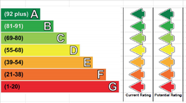
I've placed all the arrows in the cells they are required for and they are all named arrowa, arrowb, etc with the ones in the 'potential' column are the same with a p added to the end, so arrowap.
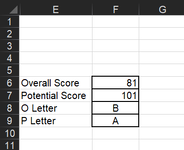
the data is on sheet2 (as per pic), i have both the score and the letter, but would assume the letter would be the easier reference to use.

i need all the arrows to disappear if the relevant letter isn't listed in F8 & F9

please help, I've tried loads of different solutions today and now i'm close to throwing the laptop out the window

thanks for any help in advance.

 

[Jaafar Tribak]

When you say "i need all the arrows to disappear if the relevant letter isn't listed in F8 & F9", what exactly do you mean by that ?

EDIT:

doesn't look like that will work either as directs to google sheets :/

No worries, I have managed to download the workbook example from the link in post#8

 

[mrbab7]

When you say "i need all the arrows to disappear if the relevant letter isn't listed in F8 & F9", what exactly do you mean by that ?

EDIT:

No worries, I have managed to download the workbook example from the link in post#8

Hi Jaafar,

Sorry since the original post i rejigged it a little, it's now referencing L12(current) & L13(potential)

to explain cells C28-C32, produce a rating, which is totalled in the two cells above, depending on the letter shown, i want it to show the relevant arrow on the chart next to it, whilst the others aren't visible.

the current VBA code has hidden all of the other 'current' arrows at the moment, but they are there the same as in 'potential'


hope this make sense

 

[Jaafar Tribak]

Ok- I think I understand but I will be logging off shortly. I will take a look later on tonight.

 

[mrbab7]

Ok- I think I understand but I will be logging off shortly. I will take a look later on tonight.

amazing, thanks in advance!

if you need to ask any more questions when you are actually looking at it, please let me know

thanks

 

[Jaafar Tribak]

Here is your revised workbook example : Energy table.xlsm

I have changed your existing code in the worsheet calculate event to make it work as required. Furthermore, I have added a couple of extra vba routines for Showing and Hiding all the Arrows and for Toggling their visibility. These extra routines are not really necessary but they may come in handy at some point... I have assigned these extra routines to 3 command buttons that I have placed accross the worksheet top as show in the preview below.

Here is the entire code in the Worksheet Module (Sheet1)

Option Explicit

Private Sub Worksheet_Calculate()
    Dim i As Long
    For i = 65 To 71
        Shapes("arrow" & Chr(i)).Visible = (UCase([L12]) = Chr(i))
        Shapes("arrow" & Chr(i) & "p").Visible = (UCase([L13]) = Chr(i))
    Next i
End Sub

Sub ToggleArrowsVisibility()
    Dim i As Long
    For i = 65 To 71
        Shapes("arrow" & Chr(i)).Visible = Not (Shapes("arrow" & Chr(i)).Visible)
        Shapes("arrow" & Chr(i) & "p").Visible = Not (Shapes("arrow" & Chr(i) & "p").Visible)
    Next i
End Sub

Sub ShowAllArrows(ByVal bShow As Boolean)
    Dim i As Long
    For i = 65 To 71
        Shapes("arrow" & Chr(i)).Visible = bShow
        Shapes("arrow" & Chr(i) & "p").Visible = bShow
    Next i
End Sub

Sub Show()
    ShowAllArrows bShow:=True
End Sub

Sub Hide()
    ShowAllArrows bShow:=False
End Sub

EDIT:
Cell D12 in Sheet1 holds the following formula: =IF(Sheet2!F5="A";"arrowa";"")
I have noticed that when the arrow above this cell D2 becomes visible, the formula evaluates to "arrowa" and the text shows underneath the arrow and slightly clutters the area. I decided to prevent the cell text from showing by setting its number format to Custom ";;;" via the Format Cells Dialog>Number Tab. You can change this if you want.

 

[mrbab7]

Here is your revised workbook example : Energy table.xlsm

I have changed your existing code in the worsheet calculate event to make it work as required. Furthermore, I have added a couple of extra vba routines for Showing and Hiding all the Arrows and for Toggling their visibility. These extra routines are not really necessary but they may come in handy at some point... I have assigned these extra routines to 3 command buttons that I have placed accross the worksheet top as show in the preview below.


View attachment 77938



Here is the entire code in the Worksheet Module (Sheet1)

Option Explicit

Private Sub Worksheet_Calculate()
    Dim i As Long
    For i = 65 To 71
        Shapes("arrow" & Chr(i)).Visible = (UCase([L12]) = Chr(i))
        Shapes("arrow" & Chr(i) & "p").Visible = (UCase([L13]) = Chr(i))
    Next i
End Sub

Sub ToggleArrowsVisibility()
    Dim i As Long
    For i = 65 To 71
        Shapes("arrow" & Chr(i)).Visible = Not (Shapes("arrow" & Chr(i)).Visible)
        Shapes("arrow" & Chr(i) & "p").Visible = Not (Shapes("arrow" & Chr(i) & "p").Visible)
    Next i
End Sub

Sub ShowAllArrows(ByVal bShow As Boolean)
    Dim i As Long
    For i = 65 To 71
        Shapes("arrow" & Chr(i)).Visible = bShow
        Shapes("arrow" & Chr(i) & "p").Visible = bShow
    Next i
End Sub

Sub Show()
    ShowAllArrows bShow:=True
End Sub

Sub Hide()
    ShowAllArrows bShow:=False
End Sub

EDIT:
Cell D12 in Sheet1 holds the following formula: =IF(Sheet2!F5="A";"arrowa";"")
I have noticed that when the arrow above this cell D2 becomes visible, the formula evaluates to "arrowa" and the text shows underneath the arrow and slightly clutters the area. I decided to prevent the cell text from showing by setting its number format to Custom ";;;" via the Format Cells Dialog>Number Tab. You can change this if you want.

Jaafar, you are a legend! this is amazing!

thank you so much!!

p.s. you were right to hide that text, i just wanted the arrow