Conditional formatting

[little dove]

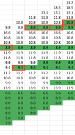
I have a spreadsheet with 100 columns and 50 rows.
I want to highlight the cells with the 8 smallest numbers in each column.

I have tried conditional formatting but it will sometimes highlights a lot more than 8 cells in each column when one of the 8 lowest is repeated.

If there is a duplicate I would like it to highlight the one in the first row it comes to (from row one working down) and then ignore duplicates.

Any help much appreciated, thanks

 

[Eric W]

Welcome to the MrExcel forum!

If your numbers are integers, it's not too hard:

Book1
	A	B	C
1	Header 1	Header 2	Header 3
2	82	29	12
3	97	14	57
4	50	25	49
5	41	61	99
6	58	54	27
7	1	84	95
8	67	61	65
9	78	33	21
10	38	67	70
11	37	57	87
12	93	23	9
13	8	93	47
14	67	84	36
15	86	66	40
16	19	55	84
17	4	66	77
18	55	91	38
19	94	74	8
20	10	85	15
21	75	77	24
22	39	95	52
23	1	32	2
24	65	45	53
25	65	96	28
26	51	12	42
27	56	88	100
28	56	14	63
29	64	57	57
30	85	87	16
31	26	39	35
32	21	13	80
33	52	52	10
34	91	45	25
35	35	70	16
36	53	96	60
37	11	77	15
38	96	22	76
39	8	21	28
40	8	73	15
41	56	56	88
42	82	72	94
43	77	91	94
44	11	35	95
45	49	55	51
46	72	68	12
47	75	4	10
48	12	9	64
49	14	40	5
50	68	90	45
51	32	12	1
52
Sheet1

Cells with Conditional Formatting
Cell	Condition		Cell Format	Stop If True
A2:C51	Expression	=A2+ROW(A2)/100<=SMALL(A$2:A$51+ROW(A$2:A$51)/100,8)	text	NO

If they're not integers, it gets harder since we need to include some COUNTIF terms. Let me know how this works.

 

[little dove]

thanks, but cant see how that works. You have highlighted two cells with the same number in column A. Also unfortunately the numbers are to 1 decimal place.
In my example I did the formatting manually. As you can see I am highlighting 8 cells in each column. In the right hand colum I only highlight the 10.8 nearest the top. Other 10.8’s are ignored. The cell with the red border is my next enhancement. I also want to identify if possible the highest of the selected 8.

 

[Snakehips]

@little dove I believe that Excel 2021 supports the UNIQUE function.
If so then maybe like below.

Book2
	A	B	C
1	11	11	11
2	2	13	6
3	3	3	6
4	4	4	6.5
5	5	5	6
6	6	6	5.3
7	7	7	7
8	7	7	2
9	7	7	7
10	-2	-2	-2
11	8	8	8
12	9	9	9
13	10	10	10
14	11	11	11
15	12	12	12
16	13	13	13
17	1	1	1
18	1	1	1
19	1	1	1
20	1	1	1
21	1	1	1
22	1	1	1
23	1	1	1
24	1	1	1
25	1	1	1
26	1	1	1
27	1	1	2
28	1	1	1
29	1	1	1
30	1	1	1
31	1	1	1
32	1	1	1
33	1	1	1
34	1	1	1
35	1	1	1
36	1	1	1
37	1	1	1
38	1	1	1
39	1	1	1
40	1	1	1
41	1	1	1
42	1	1	1
43	1	1	1
44	1	1	1
45	1	1	1
46	1	1	1
47	1	1	1
48	1	1	1
49	1	1	1
50	1	1	1
Sheet2

Cells with Conditional Formatting
Cell	Condition		Cell Format	Stop If True
A1:Y50	Expression	=AND(A1<>"",A1<=SMALL(UNIQUE(A$1:A$50,,),8),ROWS(A$1:A1),COUNTIF(A$1:A1,A1)=1)	text	NO

Hope that helps.

 

[little dove]

I am such an idiot. misunderstood my brief. duplicates are ok, but only as long as no more than 8 cells are highlighted. sorry. How do I do this please?

 

[Eric W]

My original post allowed duplicates, but only highlighted 8 cells maximum. I misunderstood your original question, but it sounds like that's what you want after all. That formula might work for you if you change the 100's to 10000's, but that depends on whether your values are exactly 1 decimal place, or if there are more that aren't showing. Here's another method that should work no matter how many decimals there are:

Book1
	A	B	C
1	Header 1	Header 2	Header 3
2	10.1	11	7.2
3	14.3	12.5	7.8
4	18.5	6.7	11.3
5	10.1	6.1	14.8
6	9.2	8	9
7	9.3	18.9	16.3
8	6.5	5.2	10.5
9	15.1	10.2	12.7
10	19.1	14.1	7.9
11	17.5	7.2	9.4
12	8.7	18.2	15
13	11.5	14.2	14.8
14	19.6	6.3	19.5
15	5.7	16.1	13.6
16	12.7	7.4	18
17	8	11.6	5
18	6	10.5	15.6
19	16.1	13.7	13
20	20	6.4	5.7
21	12.6	5.8	14.1
22	8.7	19.6	7.5
23	6.5	5.1	16.4
24	6	11.3	9.6
25	7.6	7.3	11.1
26	16.7	13.6	12.5
27	11.1	10	14.6
28	14.2	5.8	13.9
29	18.7	18.7	6.3
30	12.6	13.3	14.5
31	9.7	5.3	15.9
32	18.6	14.5	16.5
33	17	17.2	16
34	8.1	6.1	13.6
35	8.9	18.4	17.9
36	18	13.4	5.8
37	8.2	14.6	6.8
38	6	18.8	13.8
39	19.1	15.7	6.8
40	13.3	16.4	11.8
41	18.9	15.1	17
42	15.4	13.4	5.8
43	7.9	14.1	12.7
44	11.5	16.8	9.4
45	14.9	6.3	13.2
46	18.9	5	19.1
47	8	15.2	9.7
48	6	9.9	10.6
49	15.4	13	13.8
50	13	19.6	17.6
51	10	8.6	15.6
Sheet1

Cells with Conditional Formatting
Cell	Condition		Cell Format	Stop If True
A2:C51	Expression	=MATCH(ROW(A2),SORTBY(ROW(A$2:A$51),A$2:A$51),0)=8	text	NO
A2:C51	Expression	=MATCH(ROW(A2),SORTBY(ROW(A$2:A$51),A$2:A$51),0)<=8	text	NO

Conditional Formatting doesn't allow the really heavy outlining, so the red outline doesn't show up really well. Maybe you just highlight the cell in red.

 

[little dove]

Thanks again. I tried but it didn't work for me.

WHS Golf handicap.xlsx
	V
17
Scores

Cells with Conditional Formatting
Cell	Condition		Cell Format	Stop If True
Q6:AJ50	Expression	=MATCH(ROW(Q6),SORTBY(ROW(Q$6:Q50),Q$6:Q$50),0)=8	text	NO
Q6:AJ50	Expression	=MATCH(ROW(Q6),SORTBY(ROW(Q$6:Q50),Q$6:Q$50),0)<=8	text	NO

 

[little dove]

It works. thank you so much

 

[little dove]

"Conditional Formatting doesn't allow the really heavy outlining, so the red outline doesn't show up really well. Maybe you just highlight the cell in red."
So I just need to change the format on the highest of the highlighted 8 numbers to a different colour. How do I do this please?

 

[little dove]

Please ignore my last. I have realised what the formulas do. My final word. thanks so much!!!!!!!