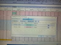
Conditional formatting

[Dhudson]

So what I'm trying to do is for example

The information in D, E and F column are fixed.

but the colour of the number is conditional to the DEF column so

• G is conditional to D
  • G4 to D4
  • G5 to D5 etc
• H is conditional to E
• I is conditional to F

If it is higher than the previous number then the box turns red and if it is lower it turns green. This bit I have worked out

Is there a quick way to format the entire table or does it have to be conditioned for each cell? There’s over 3000 cells to format.

Is there no way to copy the layout of the entire format and move its position across to the right one or to cells below

 

[aRandomHelper]

Hi, welcome to the forums.

Conditional formatting can be "relatively formatted". E.g. if I want a red applied to range A1:B20 if any cell is >0, I can choose that range, and only use the rule =A1>0 (use the top left cell address as first-cell reference).
For your case, maybe use D1 / E1 / F1 respectively for the conditions used in column G / H / I respectively.

 

[Dhudson]

Hi, welcome to the forums.

Conditional formatting can be "relatively formatted". E.g. if I want a red applied to range A1:B20 if any cell is >0, I can choose that range, and only use the rule =A1>0 (use the top left cell address as first-cell reference).
For your case, maybe use D1 / E1 / F1 respectively for the conditions used in column G / H / I respectively.

Would this work if I wanted them conditional to certain cells

So G4 to D4
G5 to G5 etc

 

[Fluff]

Yes, select G4 to I last row & then apply the conditional formatting using

=G4<D4

 

[Dhudson]

Can you explain where I do all of this. I’m not sure of where to find all of this

 

[Fluff]

Select the cells, then on the home tabe select conditional formatting, new rule, use a formula & use the formula I posted.

 

[Dhudson]

I tried that and it seemed tk still be conditionally formatted tk the box at the top of the spreadsheet

Is there no way of duplicating this format multiple times but so that the whole format moves or a way of doing it for the whole column but still relative to the cell three to the left still for the whole column

 

[Fluff]

That image is totally unreadable.

 

[Dhudson]

That image is totally unreadable.

It won’t let me upload the image’s actual size

 

[Fluff]

Did you select the entire range to be formatted, or just a single cell?