Conditionally format the last cell in each row with valuable data

paydog23

New Member
Joined
Jul 12, 2017
Messages
28
Office Version
  1. 365
Platform
  1. Windows
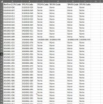
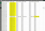
I have a dataset for wells and 5 treatment plants (TP1, TP2, TP3, TP4, and TP5), which extends from A1 to F841. The flow path for each well is such that the well flows to TP1, then TP2, and so on. However, sometimes the flow path does not extend all the way to TP5. I have manually entered "None" in the cells corresponding to the non-existent TP2s, TP3s, TP4s, and TP5s. However, I would like to conditionally format or automatically color the last cell in each row that does have a TP PS Code (i.e. 0110010-020, instead of none). I have uploaded 2 pictures. The first picture shows the dataset I have and the second picture shows my desired output (I have manually filled in the cells yellow).
 

Attachments

  • Conditional Format Last Cell with Real Data 1.jpg
    Conditional Format Last Cell with Real Data 1.jpg
    112.7 KB · Views: 15
  • Desired Output.jpg
    Desired Output.jpg
    81.3 KB · Views: 16

Excel Facts

What is the shortcut key for Format Selection?
Ctrl+1 (the number one) will open the Format dialog for whatever is selected.
I don't feel like typing in that data, so all I can help you with is a video about conditional formatting that might benefit you in your efforts.
ExcelIsFun_CF
 
Upvote 0
I don't feel like typing in that data,
@paydog23
I agree with DRSteele. Suggest you look at the links in my signature block below for a good way to provide sample copyable data.

Try selecting B2:F841 and apply the Conditional Formatting shown below.

Book1
BCDEF
2NoneNoneNoneNoneNone
3xxNoneNoneNone
4NoneNoneNoneNoneNone
5NoneNoneNoneNoneNone
6xNoneNoneNoneNone
7xNoneNoneNoneNone
8xxxxNone
9xNoneNoneNoneNone
10xNoneNoneNoneNone
11xNoneNoneNoneNone
12xxxxx
Sheet2 (2)
Cells with Conditional Formatting
CellConditionCell FormatStop If True
B2:F13Expression=COUNTIF(B2:$F2,"<>None")=1textNO
 
Upvote 0
@paydog23
I agree with DRSteele. Suggest you look at the links in my signature block below for a good way to provide sample copyable data.

Try selecting B2:F841 and apply the Conditional Formatting shown below.

Book1
BCDEF
2NoneNoneNoneNoneNone
3xxNoneNoneNone
4NoneNoneNoneNoneNone
5NoneNoneNoneNoneNone
6xNoneNoneNoneNone
7xNoneNoneNoneNone
8xxxxNone
9xNoneNoneNoneNone
10xNoneNoneNoneNone
11xNoneNoneNoneNone
12xxxxx
Sheet2 (2)
Cells with Conditional Formatting
CellConditionCell FormatStop If True
B2:F13Expression=COUNTIF(B2:$F2,"<>None")=1textNO

Thanks, but unfortunately, this code ended up formatting incorrect cells too, including all of column F.
 
Upvote 0
Thanks, but unfortunately, this code ended up formatting incorrect cells too, including all of column F.
Actually, I found out what the issue was--I extended the countif range to column A, and then it formatted correctly.
 
Upvote 0
Actually, I found out what the issue was--I extended the countif range to column A, and then it formatted correctly.
If you have it working that is fine, but I think the actual issue was not with the CF formula range but you didn't apply it as suggested:
Try selecting B2:F841 and apply the Conditional Formatting shown below.
If you selected A2:F841 then the CF formula I suggested would act incorrectly just as you described. :)
 
Upvote 0

Forum statistics

Threads
1,214,892
Messages
6,122,112
Members
449,066
Latest member
Andyg666

We've detected that you are using an adblocker.

We have a great community of people providing Excel help here, but the hosting costs are enormous. You can help keep this site running by allowing ads on MrExcel.com.
Allow Ads at MrExcel

Which adblocker are you using?

Disable AdBlock

Follow these easy steps to disable AdBlock

1)Click on the icon in the browser’s toolbar.
2)Click on the icon in the browser’s toolbar.
2)Click on the "Pause on this site" option.
Go back

Disable AdBlock Plus

Follow these easy steps to disable AdBlock Plus

1)Click on the icon in the browser’s toolbar.
2)Click on the toggle to disable it for "mrexcel.com".
Go back

Disable uBlock Origin

Follow these easy steps to disable uBlock Origin

1)Click on the icon in the browser’s toolbar.
2)Click on the "Power" button.
3)Click on the "Refresh" button.
Go back

Disable uBlock

Follow these easy steps to disable uBlock

1)Click on the icon in the browser’s toolbar.
2)Click on the "Power" button.
3)Click on the "Refresh" button.
Go back
Back
Top