Consolidate Data and Sum Value

[JMJ]

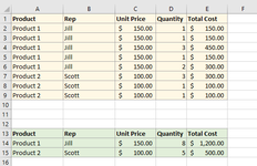
Hi, I would like to take the data in the yellow table and make it look like the green table. I tried using Consolidate, but I lose the Rep column and the Unit Price column gets summed. Product, Rep, and Unit Price could be considered a unique identifier. For all the rows in which they are the same, I only need them listed once and would like a their Quantity and Total Cost to be summed as shown in the green table. I don't work with excel much and haven't found an answer to this specific question online. I am using Excel 365.
Thanks for any help you can provide!

 

[lrobbo314]

Book1
	A	B	C	D	E
1	Product	Rep	Unit Price	Quantity	Total Cost
2	Product 1	Jill	$150.00	1	$150.00
3	Product 1	Jill	$150.00	1	$150.00
4	Product 1	Jill	$150.00	3	$450.00
5	Product 1	Jill	$150.00	1	$150.00
6	Product 1	Jill	$150.00	2	$300.00
7	Product 2	Scott	$100.00	3	$300.00
8	Product 2	Scott	$100.00	1	$100.00
9	Product 2	Scott	$100.00	1	$100.00
10
11	Product	Rep	Unit Price	Quantity	Total Cost
12	Product 1	Jill	$150.00	8	$1,200.00
13	Product 2	Scott	$100.00	5	$500.00
Sheet6

Cell Formulas
Range	Formula
A12:E13	A12	=LET(pr,UNIQUE(B2:B9),p,UNIQUE(A2:A9),up,UNIQUE(C2:C9),q,SUMIF(A2:A9,p,D2:D9),tc,SUMIF(A2:A9,p,E2:E9),CHOOSE({1,2,3,4,5},p,pr,up,q,tc))
Dynamic array formulas.

 

[lrobbo314]

This version is a bit better. I made the initial table into an actual table so when new data is added below it the formula will pick up the new values. And I tweaked the formula a bit too.

Book1
	A	B	C	D	E	F	G	H	I	J	K	L
1	Product	Rep	Unit Price	Quantity	Total Cost			Product	Rep	Unit Price	Quantity	Total Cost
2	Product 1	Jill	$150.00	1	$150.00			Product 1	Jill	$150.00	8	$1,200.00
3	Product 1	Jill	$150.00	1	$150.00			Product 2	Scott	$100.00	6	$600.00
4	Product 1	Jill	$150.00	3	$450.00			Product 3	Bill	$200.00	14	$2,800.00
5	Product 1	Jill	$150.00	1	$150.00
6	Product 1	Jill	$150.00	2	$300.00
7	Product 2	Scott	$100.00	4	$300.00
8	Product 2	Scott	$100.00	1	$100.00
9	Product 2	Scott	$100.00	1	$100.00
10	Product 3	Bill	$200.00	4	$100.00
11	Product 3	Bill	$200.00	2	$100.00
12	Product 3	Bill	$200.00	8	$100.00
Sheet6

Cell Formulas
Range	Formula
H2:L4	H2	=LET(a,Table6[Product],b,Table6[Rep],c,Table6[Unit Price],d,Table6[Quantity],e,Table6[Total Cost],pr,UNIQUE(a),r,UNIQUE(b),up,UNIQUE(c),q,SUMIF(a,pr,d),tc,up*q,CHOOSE({1,2,3,4,5},pr,r,up,q,tc))
Dynamic array formulas.

 

[JMJ]

Thank you for fixing my example spreadsheet and for the formula! Now I need to adjust it and try it on my real spreadsheet which has a few additional columns and about 13,000 rows.

 

[JMJ]

This version is a bit better. I made the initial table into an actual table so when new data is added below it the formula will pick up the new values. And I tweaked the formula a bit too.

Book1
	A	B	C	D	E	F	G	H	I	J	K	L
1	Product	Rep	Unit Price	Quantity	Total Cost			Product	Rep	Unit Price	Quantity	Total Cost
2	Product 1	Jill	$150.00	1	$150.00			Product 1	Jill	$150.00	8	$1,200.00
3	Product 1	Jill	$150.00	1	$150.00			Product 2	Scott	$100.00	6	$600.00
4	Product 1	Jill	$150.00	3	$450.00			Product 3	Bill	$200.00	14	$2,800.00
5	Product 1	Jill	$150.00	1	$150.00
6	Product 1	Jill	$150.00	2	$300.00
7	Product 2	Scott	$100.00	4	$300.00
8	Product 2	Scott	$100.00	1	$100.00
9	Product 2	Scott	$100.00	1	$100.00
10	Product 3	Bill	$200.00	4	$100.00
11	Product 3	Bill	$200.00	2	$100.00
12	Product 3	Bill	$200.00	8	$100.00
Sheet6

Cell Formulas
Range	Formula
H2:L4	H2	=LET(a,Table6[Product],b,Table6[Rep],c,Table6[Unit Price],d,Table6[Quantity],e,Table6[Total Cost],pr,UNIQUE(a),r,UNIQUE(b),up,UNIQUE(c),q,SUMIF(a,pr,d),tc,up*q,CHOOSE({1,2,3,4,5},pr,r,up,q,tc))
Dynamic array formulas.

Thanks again for replying! I just realized there is one part of my scenario that I did not explain very well. The same Product can be associated with more than one Rep. Basically, the combination of Product and Rep make a unique identifier. I need to alter the UNIQUE part of the formula. I totally understand if you don't feel like helping again.

SIMStest.xlsx
	A	B	C	D	E	F	G	H	I	J	K
1	Product	Rep	Unit Price	Quantity	Total Cost		Product	Rep	Unit Price	Quantity	Total Cost
2	Product 1	Jill	$ 150.00	1	$ 150.00		Product 1	Jill	$ 150.00	5	$ 750.00
3	Product 1	Jill	$ 150.00	1	$ 150.00		Product 2	Jill	$ 200.00	2	$ 400.00
4	Product 1	Jill	$ 150.00	3	$ 450.00		Product 2	Scott	$ 100.00	5	$ 500.00
5	Product 2	Jill	$ 200.00	2	$ 400.00		Product 1	Bill	$ 50.00	3	$ 150.00
6	Product 2	Scott	$ 100.00	3	$ 300.00		Product 3	Bill	$ 25.00	4	$ 100.00
7	Product 2	Scott	$ 100.00	1	$ 100.00
8	Product 2	Scott	$ 100.00	1	$ 100.00
9	Product 1	Bill	$ 50.00	3	$ 150.00
10	Product 3	Bill	$ 25.00	1	$ 25.00
11	Product 3	Bill	$ 25.00	3	$ 75.00
Sheet2 (3)

 

[lrobbo314]

Don't know if that can be done with a single cell formula like the last one, but this seems to do it.

Book1
	A	B	C	D	E	F	G	H	I	J	K
1	Product	Rep	Unit Price	Quantity	Total Cost		Product	Rep	Unit Price	Quantity	Total Cost
2	Product 1	Jill	150	1	150		Product 1	Jill	150	5	750
3	Product 1	Jill	150	1	150		Product 2	Jill	200	2	400
4	Product 1	Jill	150	3	450		Product 2	Scott	100	5	500
5	Product 2	Jill	200	2	400		Product 1	Bill	50	3	150
6	Product 2	Scott	100	3	300		Product 3	Bill	25	4	100
7	Product 2	Scott	100	1	100
8	Product 2	Scott	100	1	100
9	Product 1	Bill	50	3	150
10	Product 3	Bill	25	1	25
11	Product 3	Bill	25	3	75
Sheet7

Cell Formulas
Range	Formula
G2:I6	G2	=UNIQUE(A2:C11)
J2:J6	J2	=SUMPRODUCT(IFERROR(MATCH(A2:A11,G2,0)*MATCH(B2:B11,H2,0),0)*D2:D11)
K2:K6	K2	=I2*J2
Dynamic array formulas.

 

[lrobbo314]

Can also just make a Pivot table out of it with 'Product' and 'Rep' in the 'Rows' section and 'Unit Price', 'Quantity', and 'Total Cost' in the 'Values' section, with 'Unit Price' being calculated as minimum and the other 2 being sum.

Book1
	A	B	C	D	E
3	Product	Rep	Unit Price	Quantity	Total Cost
4	Product 1	Bill	50	3	150
5		Jill	150	5	750
6	Product 2	Jill	200	2	400
7		Scott	100	5	500
8	Product 3	Bill	25	4	100
9	Grand Total		25	19	1900
Sheet8

 

[JMJ]

Thanks so much for the help! I appreciate it!

 

[lrobbo314]

1 cell formula.

Book One.xlsx
	A	B	C	D	E	F	G	H	I	J	K
1	Product	Rep	Unit Price	Quantity	Total Cost		Product	Rep	Unit Price	Quantity	Total Cost
2	Product 1	Jill	150	1	150		Product 1	Jill	150	5	750
3	Product 1	Jill	150	1	150		Product 2	Jill	200	2	400
4	Product 1	Jill	150	3	450		Product 2	Scott	100	5	500
5	Product 2	Jill	200	2	400		Product 1	Bill	50	3	150
6	Product 2	Scott	100	3	300		Product 3	Bill	25	4	100
7	Product 2	Scott	100	1	100
8	Product 2	Scott	100	1	100
9	Product 1	Bill	50	3	150
10	Product 3	Bill	25	1	25
11	Product 3	Bill	25	3	75
Sheet4

Cell Formulas
Range	Formula
G2:K6	G2	=LET(tbl,UNIQUE(TBL[[Product]:[Unit Price]]),p,INDEX(tbl,,1),r,INDEX(tbl,,2),qc,TBL[Quantity],tc,TBL[Total Cost],pc,TBL[Product],rc,TBL[Rep],q,SUMIFS(qc,pc,p,rc,r),up,INDEX(tbl,,3),t,up*q,CHOOSE({1,2,3,4,5},p,r,up,q,t))
Dynamic array formulas.

 

[JMJ]

1 cell formula.

Book One.xlsx
	A	B	C	D	E	F	G	H	I	J	K
1	Product	Rep	Unit Price	Quantity	Total Cost		Product	Rep	Unit Price	Quantity	Total Cost
2	Product 1	Jill	150	1	150		Product 1	Jill	150	5	750
3	Product 1	Jill	150	1	150		Product 2	Jill	200	2	400
4	Product 1	Jill	150	3	450		Product 2	Scott	100	5	500
5	Product 2	Jill	200	2	400		Product 1	Bill	50	3	150
6	Product 2	Scott	100	3	300		Product 3	Bill	25	4	100
7	Product 2	Scott	100	1	100
8	Product 2	Scott	100	1	100
9	Product 1	Bill	50	3	150
10	Product 3	Bill	25	1	25
11	Product 3	Bill	25	3	75
Sheet4

Cell Formulas
Range	Formula
G2:K6	G2	=LET(tbl,UNIQUE(TBL[[Product]:[Unit Price]]),p,INDEX(tbl,,1),r,INDEX(tbl,,2),qc,TBL[Quantity],tc,TBL[Total Cost],pc,TBL[Product],rc,TBL[Rep],q,SUMIFS(qc,pc,p,rc,r),up,INDEX(tbl,,3),t,up*q,CHOOSE({1,2,3,4,5},p,r,up,q,t))
Dynamic array formulas.

This is even better, thanks!!