Convert Unconventional D:H:M Counter to Total Minutes

jkerekgyarto

New Member
Joined
Jan 5, 2021
Messages
5
Office Version
  1. 365
Platform
  1. Windows
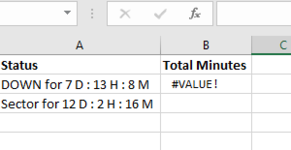
I need to convert these cells that contain elapsed time in the format shown, to total minutes.

The data in the cell is texts and numbers – there is a space on both sides of each number.

The formula is a Value function with a nested Find – it’s not working for me, however.

=VALUE(LEFT(A2,FIND("D",A2)-2))*24*60 + VALUE(LEFT(A2,FIND("D",A2)-3))*24*60 + VALUE(MID(A2,FIND(":",A2)+2,FIND("H",A2)-2))*60 + VALUE(LEFT(A2,FIND("M",A2)-2))

The position of the characters in the cells is not static – see the difference between A2 and A3.

Image of cells in spreadsheet is uploaded.

Any help is very appreciated.
 

Attachments

  • Screenshot 2021-01-05 151313.png
    Screenshot 2021-01-05 151313.png
    5.2 KB · Views: 10

Excel Facts

How can you automate Excel?
Press Alt+F11 from Windows Excel to open the Visual Basic for Applications (VBA) editor.
maybe
rawMinutes
D : 13 H : 8 M 788
2 D : 2 H : 16 M 3016

Power Query:
// Table1
let
    Source = Excel.CurrentWorkbook(){[Name="Table1"]}[Content],
    TS = Table.AddColumn(Source, "Custom", each Text.Select([raw], {"0".."9",":"})),
    Split = Table.SplitColumn(TS, "Custom", Splitter.SplitTextByEachDelimiter({":"}, QuoteStyle.Csv, false), {"Custom.1", "Custom.2"}),
    TCC = Table.CombineColumns(Split,{"Custom.1", "Custom.2"},Combiner.CombineTextByDelimiter(".", QuoteStyle.None),"Merged"),
    Trim = Table.AddColumn(TCC, "Minutes", each Text.Trim([Merged], ".")),
    Suffix = Table.TransformColumns(Trim, {{"Minutes", each _ & ":00", type text}}),
    Duration = Table.TransformColumnTypes(Suffix,{{"Minutes", type duration}}),
    Minutes = Table.TransformColumns(Duration,{{"Minutes", Duration.TotalMinutes, type number}}),
    TSC = Table.SelectColumns(Minutes,{"Minutes"})
in
    TSC
would be better if you post representative example using XL2BB not a picture
 
Upvote 0
You may try this method.

1609887562576.png


Enter the following formula in B1 BS and copy it down.

=IFERROR(IFERROR(MID(SUBSTITUTE(A1," ",""),1,FIND("D",SUBSTITUTE(A1," ",""))-1)*24*60,0)+IFERROR(MID(SUBSTITUTE(A1," ",""),FIND(":",SUBSTITUTE(A1," ",""))+1,FIND("H",SUBSTITUTE(A1," ",""))-1-FIND(":",SUBSTITUTE(A1," ","")))*60,0)+MID(SUBSTITUTE(A1," ",""),FIND("H",SUBSTITUTE(A1," ",""))+2,FIND("M",SUBSTITUTE(A1," ",""))-1-FIND("H",SUBSTITUTE(A1," ",""))-1),0)


Kind regards

Saba
 
Upvote 0
maybe
rawMinutes
D : 13 H : 8 M 788
2 D : 2 H : 16 M 3016

Power Query:
// Table1
let
    Source = Excel.CurrentWorkbook(){[Name="Table1"]}[Content],
    TS = Table.AddColumn(Source, "Custom", each Text.Select([raw], {"0".."9",":"})),
    Split = Table.SplitColumn(TS, "Custom", Splitter.SplitTextByEachDelimiter({":"}, QuoteStyle.Csv, false), {"Custom.1", "Custom.2"}),
    TCC = Table.CombineColumns(Split,{"Custom.1", "Custom.2"},Combiner.CombineTextByDelimiter(".", QuoteStyle.None),"Merged"),
    Trim = Table.AddColumn(TCC, "Minutes", each Text.Trim([Merged], ".")),
    Suffix = Table.TransformColumns(Trim, {{"Minutes", each _ & ":00", type text}}),
    Duration = Table.TransformColumnTypes(Suffix,{{"Minutes", type duration}}),
    Minutes = Table.TransformColumns(Duration,{{"Minutes", Duration.TotalMinutes, type number}}),
    TSC = Table.SelectColumns(Minutes,{"Minutes"})
in
    TSC
would be better if you post representative example using XL2BB not a picture
Thank you for your response - I was able download the add-in

LSOD Dashboard.xlsm
AB
1StatusTotal Minutes
2DOWN for 7 D : 13 H : 8 M#VALUE!
3Sector for 12 D : 2 H : 16 M
Sheet1
Cell Formulas
RangeFormula
B2B2=VALUE(LEFT(A2,FIND("D",A2)-2))*24*60 + VALUE(LEFT(A2,FIND("D",A2)-3))*24*60 + VALUE(MID(A2,FIND(":",A2)+2,FIND("H",A2)-2))*60 + VALUE(LEFT(A2,FIND("M",A2)-2))


does the words "down" and "sector" make difference? I am not sure how to implement your solution.
 
Upvote 0
You may try this method.

View attachment 29131

Enter the following formula in B1 BS and copy it down.

=IFERROR(IFERROR(MID(SUBSTITUTE(A1," ",""),1,FIND("D",SUBSTITUTE(A1," ",""))-1)*24*60,0)+IFERROR(MID(SUBSTITUTE(A1," ",""),FIND(":",SUBSTITUTE(A1," ",""))+1,FIND("H",SUBSTITUTE(A1," ",""))-1-FIND(":",SUBSTITUTE(A1," ","")))*60,0)+MID(SUBSTITUTE(A1," ",""),FIND("H",SUBSTITUTE(A1," ",""))+2,FIND("M",SUBSTITUTE(A1," ",""))-1-FIND("H",SUBSTITUTE(A1," ",""))-1),0)


Kind regards

Saba
I am new and didn't have the add-in installed - Here is the complete cell contents - Each cell will have various words like "DOWN" "Sector" "UP" - Does this make a difference to your solution?

LSOD Dashboard.xlsm
AB
1StatusTotal Minutes
2DOWN for 7 D : 13 H : 8 M#VALUE!
3Sector for 12 D : 2 H : 16 M
Sheet1
Cell Formulas
RangeFormula
B2B2=VALUE(LEFT(A2,FIND("D",A2)-2))*24*60 + VALUE(LEFT(A2,FIND("D",A2)-3))*24*60 + VALUE(MID(A2,FIND(":",A2)+2,FIND("H",A2)-2))*60 + VALUE(LEFT(A2,FIND("M",A2)-2))
 
Upvote 0
You may try this method.

View attachment 29131

Enter the following formula in B1 BS and copy it down.

=IFERROR(IFERROR(MID(SUBSTITUTE(A1," ",""),1,FIND("D",SUBSTITUTE(A1," ",""))-1)*24*60,0)+IFERROR(MID(SUBSTITUTE(A1," ",""),FIND(":",SUBSTITUTE(A1," ",""))+1,FIND("H",SUBSTITUTE(A1," ",""))-1-FIND(":",SUBSTITUTE(A1," ","")))*60,0)+MID(SUBSTITUTE(A1," ",""),FIND("H",SUBSTITUTE(A1," ",""))+2,FIND("M",SUBSTITUTE(A1," ",""))-1-FIND("H",SUBSTITUTE(A1," ",""))-1),0)


Kind regards

Saba
Saba - This formula is converting the hours and minutes but not the days - see below..

LSOD Dashboard.xlsm
AB
1StatusTotal Minutes
2DOWN for 7 D : 13 H : 8 M788
3Sector for 12 D : 2 H : 16 M136
Sheet1
Cell Formulas
RangeFormula
B2:B3B2=IFERROR(IFERROR(MID(SUBSTITUTE(A2," ",""),1,FIND("D",SUBSTITUTE(A2," ",""))-1)*24*60,0)+IFERROR(MID(SUBSTITUTE(A2," ",""),FIND(":",SUBSTITUTE(A2," ",""))+1,FIND("H",SUBSTITUTE(A2," ",""))-1-FIND(":",SUBSTITUTE(A2," ","")))*60,0)+MID(SUBSTITUTE(A2," ",""),FIND("H",SUBSTITUTE(A2," ",""))+2,FIND("M",SUBSTITUTE(A2," ",""))-1-FIND("H",SUBSTITUTE(A2," ",""))-1),0)
 
Upvote 0
I added a helper column to solve problem.

1609890495166.png


Enter the following formula in B1 and copy it down

=SUBSTITUTE(SUBSTITUTE(SUBSTITUTE(A1," ",""),"Downfor",""),"Sectorfor","")

And enter the following formula in C1 and copy it down.

=IFERROR(IFERROR(MID(B1,1,FIND("D",B1,2)-1)*24*60,0)+IFERROR(MID(B1,FIND(":",B1)+1,FIND("H",B1)-1-FIND(":",B1))*60,0)+MID(B1,FIND("H",B1)+2,FIND("M",B1)-1-FIND("H",B1)-1),0)

Kind regards

Saba
 
Upvote 0
Solution
Just a guess without a clear and useful example.

T202101a.xlsm
AB
1DataMinutes
2 D : 13 H : 8 M 788
3 2 D : 2 H : 16 M 3016
4 D : 2 H : 16 M 136
3b
Cell Formulas
RangeFormula
B2:B4B2=IF(ISNUMBER(--LEFT(A2,2)),LEFT(A2,2)*24*60+MID(A2,FIND(":",A2)+2,2)*60+MID(A2,FIND("M",A2)-3,2),MID(A2,FIND(":",A2)+2,2)*60+MID(A2,FIND("M",A2)-3,2))
 
Upvote 0
I added a helper column to solve problem.

View attachment 29133

Enter the following formula in B1 and copy it down

=SUBSTITUTE(SUBSTITUTE(SUBSTITUTE(A1," ",""),"Downfor",""),"Sectorfor","")

And enter the following formula in C1 and copy it down.

=IFERROR(IFERROR(MID(B1,1,FIND("D",B1,2)-1)*24*60,0)+IFERROR(MID(B1,FIND(":",B1)+1,FIND("H",B1)-1-FIND(":",B1))*60,0)+MID(B1,FIND("H",B1)+2,FIND("M",B1)-1-FIND("H",B1)-1),0)

Kind regards

Saba
Thank you Saba! That works nicely!
 
Upvote 0
does the words "down" and "sector" make difference? I am not sure how to implement your solution.
no, it doesn't
rawMinutes
D : 13 H : 8 M 788
2 D : 2 H : 16 M 3016
10 D : 1 H : 45 M 14505
2 H120
DOWN for 7 D : 13 H : 8 M10868
Sector for 12 D : 2 H : 16 M17416
Bla bla blabla 10 D : 1 H : 45 M blu blu Blublu14505

on Data tab - New Query find and use Blank Query then on the ribbon of Power Query Editor go to Advanced Editor and replace code there with code from the post then OK, Close&Load
for more info
 
Upvote 0

Forum statistics

Threads
1,214,382
Messages
6,119,194
Members
448,874
Latest member
Lancelots

We've detected that you are using an adblocker.

We have a great community of people providing Excel help here, but the hosting costs are enormous. You can help keep this site running by allowing ads on MrExcel.com.
Allow Ads at MrExcel

Which adblocker are you using?

Disable AdBlock

Follow these easy steps to disable AdBlock

1)Click on the icon in the browser’s toolbar.
2)Click on the icon in the browser’s toolbar.
2)Click on the "Pause on this site" option.
Go back

Disable AdBlock Plus

Follow these easy steps to disable AdBlock Plus

1)Click on the icon in the browser’s toolbar.
2)Click on the toggle to disable it for "mrexcel.com".
Go back

Disable uBlock Origin

Follow these easy steps to disable uBlock Origin

1)Click on the icon in the browser’s toolbar.
2)Click on the "Power" button.
3)Click on the "Refresh" button.
Go back

Disable uBlock

Follow these easy steps to disable uBlock

1)Click on the icon in the browser’s toolbar.
2)Click on the "Power" button.
3)Click on the "Refresh" button.
Go back
Back
Top