Copy a Cell content if a column contains a specific word.

[Thomanji]

Hi Everyone,

I am struggling with a formula to accomplish a task to concert a vertical list to a horizontal database type list.
I would be very happy if I could get some pointers on where I go wrong and how to archive my goal.

Here is the problem. I got a list like below, Cell A has a label which repeats every 11 cells. Starting with Name and End with Time Zone.

Name Text Doe1
Email me1@you.com
Operator Someone1
Product/Service name of product1
Phone 123 1234567
Company ABC Company1
Referrer URL Google
Search Engine Google
IP 210.186.133.177
Country/Region Malaysia
State Kuala Lumpur
City Kuala Lumpur[Client Info]
Language en-GB
Time Zone GMT +08
Name Text Doe2
Email me2@you.com
Operator Someone2
Product/Service name of product2
Phone 123 1234567
Company ABC Company2
Referrer URL Google
Search Engine Google
IP 210.186.133.177
Country/Region Malaysia
State Kuala Lumpur
City
Language en-GB
Time Zone GMT +08
Name Text Doe3
Email me3@you.com
Operator Someone3
Product/Service name of product3
Phone 123 1234567
Company ABC Company3
Referrer URL Google
Search Engine Google
IP
Country/Region Malaysia
State Kuala Lumpur
City Kuala Lumpur[Client Info]
Language en-GB
Time Zone GMT +08

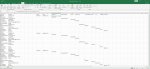
I am trying to convert this to a horizontal list with one cell per data block.

So I made a list with the horizontal values like:
Name Email Operator Product/Service Phone Company Referrer URL Search Engine Google IP Country/Region State City Language Time Zone

Than the idea is to look up Cell A and if it contains "Name" it should copy the content of Cell A2 to the cell under the name heading.
The goal is to have each vertical value under the appropriate label so that in the end this can be a CSV list of the entries.

I tried something like this for example in name
=IF(ISNUMBER(SEARCH("Name",A:A)),B:B,"") this does not work
then I did this
=IF(ISNUMBER(SEARCH("Name",A1)),B1,"")
it works but has always 11 empty cells.

=IF(ISNUMBER(SEARCH("Email",A1:A75115)),B1:B75115,"")
this works somewhat but there are some strange results. Mainly that the operator goes in the second line.

I guess there should be a better way but my formula skills are not very sophisticated and I hope that maybe someone has a tip for a better way to do this.
I have my test file attached, I do not understand why "operator" would populate the second cell and not the first. Than each next header label is another cell down.

Best wishes,
Thom

 

[Larry Haydn]

Are you familiar with VBA programming?
If so, it can be done very easily.

Your data has 14 rows for each entry.
So create the 14 headings in row 1 (in the current worksheet or a new worksheet - your choice)
Create a loop to copy each 14 rows of data, and transpose it to the blank row under your headings.
Once completed, you will have to clean up the copied data to remove the included headings: eg. State Kuala Lumpur -> Kuala Lumpur

That's it.

 

[Thomanji]

Hi Larry,

Thank you very much for taking the time to look at me issue and helping me out, I really appreciate it.
This is a good way, I did not thing of using a VBA. However my knowledge is even less with VBA.
However, I managed to get it to copy and transpose the first block but I do not understand how to loop and have it be done with the next 14 cells.

I have the following:

Sub Macro1()
'
' Macro1 Macro
'

'
Range("B1:B14").Select
Selection.Copy
Windows("Pasrse.xlsx").Activate
Range("A2").Select
Selection.PasteSpecial Paste:=xlPasteAll, Operation:=xlNone, SkipBlanks:= _
False, Transpose:=True
Windows("Parsing-vertical-list.xlsx").Activate
End Sub

But I do not know how to loop this and move the range down 14 cells on the one sheet and one cell on the paste sheet.
I would be really happy for any pointer on this.

 

[Larry Haydn]

Here is the code:

Option Explicit

Sub ProcessBrowsingData()
'==========================================
'   Split the browsing data into columns
'==========================================
Dim BData As Worksheet                              'placeholder for the worksheet name
Dim BlockFirstRow As Long, BlockLastRow As Long     'to define the first and last rows of each data block
Dim LastDataRow As Long                             'the last row of data
Dim PasteRow As Long                                'on which row to paste the data
Dim LastCopiedRow As Long                           'last row of the copied & transposed data
Dim RowNo As Long                                   'row counter, used when cleaning up the data

    '==========================================
    '   Identify this worksheet
    '   Makes reference to this sheet easier
    '==========================================
    Set BData = ActiveWorkbook.Sheets("BrowsingData")
    
    '================================
    '   Remove any existing result
    '================================
    BData.Columns("B:O").ClearContents
    
    '================================
    '   Create the column headings
    '================================
    With BData
        .Range("B1") = "Name Text"
        .Range("C1") = "Email"
        .Range("D1") = "Operator"
        .Range("E1") = "Product/Service"
        .Range("F1") = "Phone"
        .Range("G1") = "Company"
        .Range("H1") = "Referrer URL"
        .Range("I1") = "Search Engine"
        .Range("J1") = "IP"
        .Range("K1") = "Country/Region"
        .Range("L1") = "State"
        .Range("M1") = "City"
        .Range("N1") = "Language"
        .Range("O1") = "Time Zone"
    End With

    '==========================================
    '   Find the last data row
    '   so that we know when to stop copying
    '==========================================
    LastDataRow = BData.Range("A1048576").End(xlUp).Row
    
    '=============================================
    '   Specify the initial block and paste row
    '=============================================
    BlockFirstRow = 1   'Tell the program to begin copying from row 1
    BlockLastRow = 14   'Tells the program the size of the block
    PasteRow = 2
    
    '===================
    '   Begin copying
    '===================
    Do
        '================================
        '   Copy each block of 14 rows
        '================================
        BData.Range("A" & BlockFirstRow & ":A" & BlockLastRow).Copy
            '=================================
            '   Transpose the data
            '   from vertical to horizontal
            '=================================
            BData.Range("B" & PasteRow).PasteSpecial , , , True
    
        
        '================================
        '   Define the next data block
        '================================
        BlockFirstRow = BlockFirstRow + 14  'begining of next block of data
        BlockLastRow = BlockLastRow + 14    'ending of next block of data
        PasteRow = PasteRow + 1             'next row to paste the transposed data
        
    Loop Until BlockFirstRow >= LastDataRow
    
    '==============================================================
    '   Now clean up the data
    '   REPLACE removes the heading that is included in the data
    '   TRIM removes any leading- and training-spaces
    '==============================================================
    LastCopiedRow = BData.Range("B1048576").End(xlUp).Row
    
        '=======================
        '   Clean up the data
        '=======================
        For RowNo = 2 To LastCopiedRow
        
            BData.Range("B" & RowNo) = Trim(Replace(BData.Range("B" & RowNo), "Name Text", ""))
            BData.Range("C" & RowNo) = Trim(Replace(BData.Range("C" & RowNo), "Email", ""))
            BData.Range("D" & RowNo) = Trim(Replace(BData.Range("D" & RowNo), "Operator", ""))
            BData.Range("E" & RowNo) = Trim(Replace(BData.Range("E" & RowNo), "Product/Service", ""))
            BData.Range("F" & RowNo) = Trim(Replace(BData.Range("F" & RowNo), "Phone", ""))
            BData.Range("G" & RowNo) = Trim(Replace(BData.Range("G" & RowNo), "Company", ""))
            BData.Range("H" & RowNo) = Trim(Replace(BData.Range("H" & RowNo), "Referrer URL", ""))
            BData.Range("I" & RowNo) = Trim(Replace(BData.Range("I" & RowNo), "Search Engine", ""))
            BData.Range("J" & RowNo) = Trim(Replace(BData.Range("J" & RowNo), "IP", ""))
            BData.Range("K" & RowNo) = Trim(Replace(BData.Range("K" & RowNo), "Country/Region", ""))
            BData.Range("L" & RowNo) = Trim(Replace(BData.Range("L" & RowNo), "State", ""))
            BData.Range("M" & RowNo) = Trim(Replace(BData.Range("M" & RowNo), "City", ""))
            BData.Range("N" & RowNo) = Trim(Replace(BData.Range("N" & RowNo), "Language", ""))
            BData.Range("O" & RowNo) = Trim(Replace(BData.Range("O" & RowNo), "Time Zone", ""))
    
        Next RowNo
        
    '========================
    '   Format the columns
    '========================
    With BData
        .Columns("B:O").HorizontalAlignment = xlLeft
        .Columns("B:O").AutoFit
        .Range("B1").Select
    End With
        
        
End Sub

 

[Larry Haydn]

And here is the result:

VBA Samples.xlsm
	A	B	C	D	E	F	G	H	I	J	K	L	M	N	O
1	Name Text Doe1	Name Text	Email	Operator	Product/Service	Phone	Company	Referrer URL	Search Engine	IP	Country/Region	State	City	Language	Time Zone
2	Email me1@you.com	Doe1	me1@you.com	Someone1	name of product1	123 1234567	ABC 1	Google	Google	210.186.133.177	Malaysia	Kuala Lumpur	Kuala Lumpur[Client Info]	en-GB	GMT +08
3	Operator Someone1	Doe2	me2@you.com	Someone2	name of product2	123 1234567	ABC 2	Google	Google	210.186.133.177	Malaysia	Kuala Lumpur		en-GB	GMT +08
4	Product/Service name of product1	Doe3	me3@you.com	Someone3	name of product3	123 1234567	ABC 3	Google	Google		Malaysia	Kuala Lumpur	Kuala Lumpur[Client Info]	en-GB	GMT +08
5	Phone 123 1234567
6	Company ABC Company1
7	Referrer URL Google
8	Search Engine Google
9	IP 210.186.133.177
10	Country/Region Malaysia
11	State Kuala Lumpur
12	City Kuala Lumpur[Client Info]
13	Language en-GB
14	Time Zone GMT +08
BrowsingData

 

[Peter_SSs]

So I made a list with the horizontal values like:

Then you can also do this pretty easily with a formula.

Here is a smaller example (I suggest that you investigate XL2BB for providing sample data to make it easier for helpers by not having to manually type out sample data to test with. )
Hopefully you can scale it up to match your data and layout. After adjusting the ranges, copy the formula across and down.

20 05 29.xlsm
	A	B	C	D	E	F	G
1	Name	Tom		Name	Email	Operator	Company
2	Email	tom@abc.def		Tom	tom@abc.def	Someone1	Company ABC
3	Operator	Someone1		Fred	fred@aaa.com	Another operator	HHH Inc
4	Company	Company ABC		Jen	jj@aole.net.uk		Houses Plus
5	Name	Fred		Ann Thoms	a_t@home	Someone1	Big Shoes Ltd
6	Email	fred@aaa.com
7	Operator	Another operator
8	Company	HHH Inc
9	Name	Jen
10	Email	jj@aole.net.uk
11	Operator
12	Company	Houses Plus
13	Name	Ann Thoms
14	Email	a_t@home
15	Operator	Someone1
16	Company	Big Shoes Ltd
17
Vertical to Horizontal

Cell Formulas
Range	Formula
D2:G7	D2	=IFERROR(INDEX($B:$B,AGGREGATE(15,6,ROW($B$1:$B$200)/($A$1:$A$200=D$1),ROWS(D$2:D2)))&"","")

 

[Thomanji]

Larry Haydn - Wow, you are awesome. This is great, thank you very much for this.
Peter_SSs - thanks this is working too

I thank you both for your support on this. I am appreciating this assistance very much. Its nice to see that in the community we support each other.
I will pay it forward

 

[Peter_SSs]

You're welcome.

If your data is at all large and you are considering going with a macro, then this should be very fast. It assumes ..
- original data in columns A:B starting at row 1 as per your image from post #1.
- every 'block' of data has the same labels in the same order in column A.
- nothing is in column D and columns to the right

The code will automatically determine the headings required and enter them in D1, E1, F1, ...

Sub VerticalToHorizontal()
  Dim a As Variant, b As Variant
  Dim RowsPerBlock As Long, NumBlocks As Long, i As Long, j As Long, BaseNum As Long
  
  RowsPerBlock = Columns(1).Find(What:=Range("A1").Value, LookAt:=xlWhole).Row - 1
  a = Range("B1:B" & Range("A" & Rows.Count).End(xlUp).Row).Value
  NumBlocks = UBound(a) / RowsPerBlock
  ReDim b(1 To NumBlocks, 1 To RowsPerBlock)
  Do Until i = NumBlocks
    i = i + 1
    BaseNum = (i - 1) * RowsPerBlock
    For j = 1 To RowsPerBlock
      b(i, j) = a(BaseNum + j, 1)
    Next j
  Loop
  With Range("D1").Resize(, RowsPerBlock)
    .Value = Application.Transpose(Range("A1").Resize(RowsPerBlock).Value)
    .Offset(1).Resize(NumBlocks).Value = b
  End With
End Sub

 

[Larry Haydn]

Larry Haydn - Wow, you are awesome. This is great, thank you very much for this.
Peter_SSs - thanks this is working too

I thank you both for your support on this. I am appreciating this assistance very much. Its nice to see that in the community we support each other.
I will pay it forward

Many years ago (2003~2004?) I was doing an online store project with also a physical store.
The application requires integrating a barcode scanner with my application. And I have no idea how to do that.
I posted a question on some forums, and got the answer as well as the code in less than 15 minutes.

So here, I am giving back.
I hope one day you will continue this fine tradition too