Copy data to multiple sheets from data sheet with blank rows

[sauravg]

Hi, I am fairly new to VBA and trying my luck hard to get things working for me. I have an excel sheet where I am looking to get the data on a new worksheet if value matches.
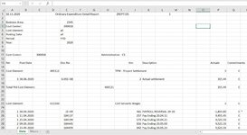
Column G has different cost centers and blank rows in between. I would like to create something if data can be read starting from the last row on column G of "DATA" tab and once a cost center starting with 30* found then it should copy the data till the next up row have a different cost center number into new worksheets including the blank rows.

For example, if Cell G435 has a cost center "30256" and the next cost center "35684" is at cell G150 then macro should start from the bottom and find the cost center number and once found, it should copy the data from G435 to G151 (even if some rows are blank) to a new worksheet and worksheet should be named as the cell value i.e. cost center.

Once the new worksheet are created, the cost center on starting with 30* should replaced by the full cost center number.

I did copy some code and changed it but it is not reflecting the result what I want to see. Below is my code.

Sub createSheets()
Dim lr As Long
Dim ws As Worksheet
Dim i As Integer
Dim ar As Variant
Dim j As Long
Dim rng As Range

Application.ScreenUpdating = False

Set ws = Sheet1 'Sheets code name
lr = ws.Range("G" & Rows.Count).End(xlUp).row
Set rng = ws.Range("G1:G" & lr)
j = ws.[A1].CurrentRegion.Columns.Count + 1
rng.AdvancedFilter 2, , ws.Cells(1, j), True
ar = ws.Range(ws.Cells(2, j), ws.Cells(Rows.Count, j).End(xlUp))

For i = 1 To UBound(ar)
rng.AutoFilter 1, ar(i, 1)
If Not Evaluate("=ISREF('" & ar(i, 1) & "'!A1)") Then
Sheets.Add(after:=Sheets(Sheets.Count)).Name = ar(i, 1)
Else
Sheets(ar(i, 1)).Move after:=Sheets(Sheets.Count)
End If
ws.Range("A1:A" & lr).Resize(, j - 1).Copy [A1]
Next

ws.AutoFilterMode = False
End Sub


I haven't added the last part to change the cost center number in different worksheet yet.

Any help is appreciated. Thanks in advance

 

[EXCEL MAX]

Hello Saurabh,
I have been studying your problem and find some solution.
Here is code that not looks as code that you show,
but works and meeting all requests from your post, except this one I do not fully understand:
( "Once the new worksheet are created, the cost center on starting with 30* should replaced by the full cost center number.")

Sub CreateSheets2()

    Dim varWS1 As Worksheet
    Dim varNRows As Long, varNRows2 As Long, varNLoops As Long
    Dim var30 As String
    Dim varNew As Byte
    
    Application.ScreenUpdating = False
    Set varWS1 = Worksheets("DATA")
    varNRows = varWS1.Range("G" & Rows.Count).End(xlUp).Row
    Sheets.Add
    For varNLoops = varNRows To 2 Step -1
         Range("G" & varNLoops).Select
         var30 = Left(varWS1.Range("G" & varNLoops), 2)
         If var30 = "30" Or IsEmpty(varWS1.Range("G" & varNLoops)) Then
            If Not IsEmpty(varWS1.Range("G" & varNLoops)) Then
                On Error GoTo EX2
                ActiveSheet.Name = varWS1.Range("G" & varNLoops).Value
                varNew = 1
            End If
            varWS1.Range("G" & varNLoops).Copy _
                Destination:=ActiveSheet.Range("A" & varNRows2 + 1)
            varNRows2 = varNRows2 + 1
         Else
            If varNew = 1 Then GoTo EX
         End If
     Next
EX:  Application.ScreenUpdating = True
     Exit Sub
EX2: MsgBox "You have sheet with this name."
     Application.DisplayAlerts = False
     ActiveSheet.Delete
     Application.ScreenUpdating = True
     
End Sub

 

[sauravg]

Hey Max,

Sorry I was on leave and just saw the update on the macro. I run your code however it says "Compile Error: Label Not Defined".

Let me simplify what I am looking from the data. I have 220 cost center in this report (28560 rows). I have these cost centers on 3 different columns however the cost center sorting criteria should be done from Column G. I have the cost center at the last row and formula should pick up the last row and copy all the rows until it finds another cost center, the flow of searching the data should be from bottom to top. I have attached the screenshot of my data tab. The column G is total of every cost center, therefore, I would like to make Column G as my data extraction column. Once the data is being copy and pasted to new worksheets, the cost center on Column E & C should also be changed as per Cost center tab. When I extract the data from SAP, The first part from row 3 to 8 remains same on each and every page of excel and once the cost center changes per column G the cost center on the new worksheet should match with header cost center. That is the reason if any code can be created when macro segregate the cost center on the basis of Column G and copy the same cost center on the header parts where it finds the value of "300018". I guess the lowest number should always come first on the report.

Hope I am able to explain you my case.

 

[EXCEL MAX]

If label is not defined it means that you need to name the line.
Add "EX:" and "EX2:" like my code shows. This meet requst from your first post.
No matter. This is the wrong approach to the problem.
Your code better describes your wishes, but not enough .
Can you upload worksheet?

 

[sauravg]

Can you see the attached worksheet ? It only has an option to upload picture files.