Copy formatting from a Range to a Cell via Drop-down list

Luiz_Wiese

New Member
Joined
Jan 2, 2020
Messages
9
Office Version
  1. 365
Platform
  1. Windows
Hello Guys,

I've been browsing for a while now and can't make it work. I've seen all the steps i need made on different threads but i can't join them due my lack of VBA syntax knowledge. Therefore I'm looking for help in the forum that helped me the most!!

I have a user colored dynamic range that i want to use as the source for the formats on a drop-down list i made via data validation. The user is going to use this code on new sheets and add new items and colors so it must be as generic as possible (I made it work with forced colors but its not what i really need :( ). I also could make it while pressing RUN on the VBE but i was hoping for an automated version, that updates whenever an item is selected on a new cell.

The steps i thought are:
1 - Compare the content of the selected item on the list to the source range with VLOOKUP;
2 - Get the addressed cell (From VLOOKUP) interior color (Maybe the whole format if going for fonts also);
3 - Apply the copied format to the selected item (Just like special paste format macros).

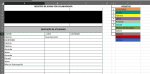
The attached image is my simplified data for now... (I've deleted lots of columns because it was originally huge [Source column on "AM" orig.] and not related to this situation)
Range A11 -> A61 Dropdown List
Range F2 -> F? Source names and formats (As extense as the user needs and as colorful too)

Thanks to all of you in advance and, if one could point me to somewhere to actively learn VBA coding I'd be more than grateful to come and help later
 

Attachments

  • ex maju.JPG
    ex maju.JPG
    96.7 KB · Views: 78

Excel Facts

Return population for a City
If you have a list of cities in A2:A100, use Data, Geography. Then =A2.Population and copy down.
Hi Luiz_Wiese, welcome to the board!

It seems clear to me what you're trying to achieve. I'm pretty sure that it's possible and I'm willing to dive into this.
Please don't expect a prompt solution and let me think about your approach for a short while.
For the basic principles of VBA: Excel Easy / TutorialsPoint
 
Upvote 0
Thanks GWteB!

I appreciate your help and I'm sure we can work on something together. I know it's not that simple thanks to the dynamic range element but I'm willing to get involved in the solution anyway I can to help... I've got some programming logic from MatLab but it is so far different from VBA that I feel completely lost. Thanks for the tips on learning also!
 
Upvote 0
Thinking further on the Issue I tried this and it worked almost perfect but it doesn't change the color everytime I select other name on the list, instead i have to run the VBE everytime I want the color updated. If we can put this code as "Always Running" mode would be my perfect scenario (I think). Here's the code.

VBA Code:
Dim Check_ROW As Variant, Cell_C As Variant
Public Sub ColorCoding()
    Cell_C = ActiveCell.Column 'Because only Column "A" has the Dropdown List

    If Cell_C = 1 Then

    Check_ROW = Application.Match(ActiveCell.Value, Range("AM:AM"), 0)
   ActiveCell.Interior.Color = Cells(Check_ROW, 39).Interior.Color

  End If

End Sub

1578083238563.png


Thanks!!!
 
Upvote 0
Hi, Luiz_Wiese. Welcome to the Board.

Try this code:
This is an Event Procedure, so you need to put it in the code module of the sheet in question (say sheet1). This is how:
Copy the code > open sheet1 > right click sheet1 tab > select View Code > paste the code.

The Sub Worksheet_Change is triggered whenever you exit a cell after you change its content.
Rich (BB code):
Private Sub Worksheet_Change(ByVal Target As Range)

If Target.Cells.CountLarge <> 1 Then Exit Sub
   If Not Intersect(Target, Range("A11:A61")) Is Nothing Then
   Dim check_row
   check_row = Application.Match(Target.Value, Range("AM:AM"), 0)
        If IsNumeric(check_row) Then
        Target.Interior.Color = Cells(check_row, 39).Interior.Color
        Else
        Target.Interior.Color = xlNone
        End If
    
    End If

End Sub
 
Upvote 0
WOW!... Thank you very much Akuini! It worked perfectly.
I do not understand the syntax and the handling of objetcs yet but I'm glad to notice I was on the right path there at least inside the If block.
 
Upvote 0
You're welcome, glad to help, & thanks for the feedback.:)

One more thing if I may ? !... I wrote edited a code to "Trim" the Data Validation for every new entry to be colored and mixed together with your work here. Can I set the "Range (A11:A61)" to be dynamic?
I was willing to close this one beautifully and consider the situation where the user would insert new rows between A11 and A61 (Or not so elegantly extend it to the 100s to overkill it).

I was thinking in something like:

Dim RNG As Range
Set RNG = "=OFFSET(A11,0,0,MATCH("TOTAL",A:A;0)-11,1))"

Since no matter what, the first is always Row11 and the last always a Row in Column A with "TOTAL" as Value

Here's the portion I put together:

VBA Code:
Private Sub Worksheet_Change(ByVal Target As Range)

 'Dim RNG As Range
 'Set RNG = "=OFFSET(A11,0,0,MATCH("TOTAL",A:A;0)-11,1))" 'Maybe here?

    If Target.Cells.CountLarge <> 1 Then Exit Sub
    If Not Intersect(Target, Range("A11:A60")) Is Nothing Then   'If Not Intersect(Target, RNG) Is Nothing Then [Is that possible??]
        Dim check_row
        check_row = Application.Match(Target.Value, Range("AM:AM"), 0)
        If IsNumeric(check_row) Then
            Target.Interior.Color = Cells(check_row, 39).Interior.Color
            
            With Target.Select
                With Selection.Validation
                    .Delete
                    .Add Type:=xlValidateList, AlertStyle:=xlValidAlertStop, Operator:= _
                         xlBetween, Formula1:="=OFFSET($AM$2,0,0,COUNTA(AM:AM),1)"
                    .IgnoreBlank = True
                    .InCellDropdown = True
                    .InputTitle = ""
                    .ErrorTitle = ""
                    .InputMessage = ""
                    .ErrorMessage = ""
                    .ShowInput = True
                    .ShowError = True
                End With
            End With
            
        Else
            Target.Interior.Color = xlNone
        End If
        
    End If
End Sub


Thanks for this last tip Akuini and it's been a pleasure to work together :)
 
Upvote 0
Since no matter what, the first is always Row11 and the last always a Row in Column A with "TOTAL" as Value
If there are no data below the cell with "TOTAL" then try replacing this line:
If Not Intersect(Target, Range("A11:A60")) Is Nothing Then
with this:
If Not Intersect(Target, Range("A11:A" & Cells(Rows.count, "A").End(xlUp).Row)) Is Nothing Then

edit:
Sorry, that won't work.
I'll try something else later.
 
Upvote 0
Try this one instead:
VBA Code:
If Not Intersect(Target, Range("A12:A" & Cells(Rows.count, "A").End(xlUp).Row).Offset(-1)) Is Nothing Then

Note: I use "A12" because it will then offset 1 row upward.
 
Upvote 0

Forum statistics

Threads
1,214,632
Messages
6,120,649
Members
448,975
Latest member
sweeberry

We've detected that you are using an adblocker.

We have a great community of people providing Excel help here, but the hosting costs are enormous. You can help keep this site running by allowing ads on MrExcel.com.
Allow Ads at MrExcel

Which adblocker are you using?

Disable AdBlock

Follow these easy steps to disable AdBlock

1)Click on the icon in the browser’s toolbar.
2)Click on the icon in the browser’s toolbar.
2)Click on the "Pause on this site" option.
Go back

Disable AdBlock Plus

Follow these easy steps to disable AdBlock Plus

1)Click on the icon in the browser’s toolbar.
2)Click on the toggle to disable it for "mrexcel.com".
Go back

Disable uBlock Origin

Follow these easy steps to disable uBlock Origin

1)Click on the icon in the browser’s toolbar.
2)Click on the "Power" button.
3)Click on the "Refresh" button.
Go back

Disable uBlock

Follow these easy steps to disable uBlock

1)Click on the icon in the browser’s toolbar.
2)Click on the "Power" button.
3)Click on the "Refresh" button.
Go back
Back
Top