Count cells in row (range) with a value that are not consecutive

jjones312

New Member
Joined
May 17, 2013
Messages
36
Office Version
  1. 365
Platform
  1. Windows
  2. MacOS
I have a spreadsheet that calculates employee absences and tardiness. There is a policy rule that if the absence is back-to-back, it only counts as a single occurrence. Currently I'm using "=COUNTIF(January[@[1]:[31]],"US")" to count all cells in a row that contains "US". Now I need to apply the policy piece.

Here is an example:
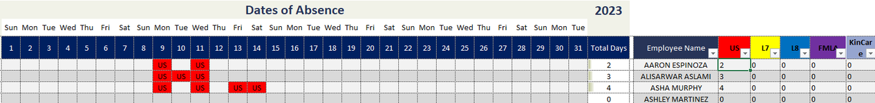
Row 1: Has entries for "US" twice on non-consecutive days. This should total in the column "US", column AK as 2 occurrences.
Row 2: Has three entries for "US" back to back, consecutive days. This should only count as 1 occurrence.
Row 3: Has four entries for "US" back-to-back and non-consecutive days. This should add up to three occurrences.

Can anyone assist in the formula for this? I'm at a lost at the moment.
 

Attachments

  • Screenshot 2023-01-10 154054.png
    Screenshot 2023-01-10 154054.png
    22.7 KB · Views: 15

Excel Facts

Can a formula spear through sheets?
Use =SUM(January:December!E7) to sum E7 on all of the sheets from January through December
Try with this UDF:

VBA Code:
Function count_absence(rng As Range, txt As String)
  Dim i As Long, n As Long
  Dim a As Variant
  Dim b As Boolean
  a = rng.Value
  b = False
  For i = 1 To UBound(a, 2)
    If UCase(a(1, i)) = UCase(txt) Then
      If b = False Then
        n = n + 1
        b = True
      End If
    ElseIf a(1, i) = "" Then
      b = False
    End If
  Next
  count_absence = n
End Function

HOW TO INSTALL UDFs
If you are new to UDFs, they are easy to install and use. To install it, simply press ALT+F11 to go into the VB editor and, once there, click Insert/Module on its menu bar, then copy/paste the above code into the code window that just opened up. That's it.... you are done. You can now use count_absence just like it was a built-in Excel function. For example:

Dante Amor
ABCDEFGHIJKLMNOPQRSTUVWXYZAAABACADAEAF
1
2sunmontuewedthufrisatsunmontuewedthufrisatsunmontuewedthufrisatsunmontuewedthufrisatsunmontue
312345678910111213141516171819202122232425262728293031Total Days
4USUS2
5USUSUS1
6USUSUSUSUSUS4
7USUSUS1
8USUSUSUS3
9USUSUS3
10USUS1
11USUSUSUSUSUSUSUSUSUSUSUSUSUSUSUSUSUSUSUSUSUSUSUSUSUSUSUSUSUSUS1
12USUSUSUSUSUSUSUSUSUSUSUSUSUSUSUSUSUSUSUSUSUSUSUSUSUSUSUSUS1
13USUSUSUSUSUSUSUSUSUSUSUSUSUSUSUSUSUSUSUSUSUSUSUSUSUSUSUSUSUS2
14USUS2
SH7
Cell Formulas
RangeFormula
AF4:AF14AF4=count_absence(January[@[1]:[31]], "US")
 
Upvote 0
What version of Excel are you using?

I suggest that you update your Account details (or click your user name at the top right of the forum) so helpers always know what Excel version(s) & platform(s) you are using as the best solution often varies by version. (Don’t forget to scroll down & ‘Save’)
 
Upvote 0
If you are using 365 or 2021 how about
Fluff.xlsm
ABCDEFGHIJKLMNOPQRSTUVWXYZAAABACADAEAFAHAIAJAK
1
2sunmontuewedthufrisatsunmontuewedthufrisatsunmontuewedthufrisatsunmontuewedthufrisatsunmontue
312345678910111213141516171819202122232425262728293031USL7
4USUSL7L7USL732
5USUSUSL7L7L7L712
6USUSUSL7L7US32
7L7USUSUSUS21
8USUSUSUS30
Temp
Cell Formulas
RangeFormula
AJ4:AK8AJ4=SUM(SIGN(IF(($B4:$AF4=AJ$3)*($A4:$AE4<>AJ$3),1,0)))
 
Upvote 0
Solution
Happy New Year to you as well.
Thanks for letting us know it works in older versions as well. (y)
 
Upvote 0
Try with this UDF:

VBA Code:
Function count_absence(rng As Range, txt As String)
  Dim i As Long, n As Long
  Dim a As Variant
  Dim b As Boolean
  a = rng.Value
  b = False
  For i = 1 To UBound(a, 2)
    If UCase(a(1, i)) = UCase(txt) Then
      If b = False Then
        n = n + 1
        b = True
      End If
    ElseIf a(1, i) = "" Then
      b = False
    End If
  Next
  count_absence = n
End Function

HOW TO INSTALL UDFs
If you are new to UDFs, they are easy to install and use. To install it, simply press ALT+F11 to go into the VB editor and, once there, click Insert/Module on its menu bar, then copy/paste the above code into the code window that just opened up. That's it.... you are done. You can now use count_absence just like it was a built-in Excel function. For example:

Dante Amor
ABCDEFGHIJKLMNOPQRSTUVWXYZAAABACADAEAF
1
2sunmontuewedthufrisatsunmontuewedthufrisatsunmontuewedthufrisatsunmontuewedthufrisatsunmontue
312345678910111213141516171819202122232425262728293031Total Days
4USUS2
5USUSUS1
6USUSUSUSUSUS4
7USUSUS1
8USUSUSUS3
9USUSUS3
10USUS1
11USUSUSUSUSUSUSUSUSUSUSUSUSUSUSUSUSUSUSUSUSUSUSUSUSUSUSUSUSUSUS1
12USUSUSUSUSUSUSUSUSUSUSUSUSUSUSUSUSUSUSUSUSUSUSUSUSUSUSUSUS1
13USUSUSUSUSUSUSUSUSUSUSUSUSUSUSUSUSUSUSUSUSUSUSUSUSUSUSUSUSUS2
14USUS2
SH7
Cell Formulas
RangeFormula
AF4:AF14AF4=count_absence(January[@[1]:[31]], "US")
This is why I come to this forum; even if there are long periods in between, everyone here is so knowledgeable and quick with the solutions. This works flawlessly, kind of. I appreciate the work, and like I said, it works perfectly, but the supervisors who use the sheet collaborate using Teams. So UDF doesn't work when posted on Teams, and they use it out of the browser. Unless there is away? I even tried to save it as an "add-in" for use, but still, when opening it in Teams, it created the #name error.

Again great work and this solution is valid.
 
Upvote 0
What version of Excel are you using?

I suggest that you update your Account details (or click your user name at the top right of the forum) so helpers always know what Excel version(s) & platform(s) you are using as the best solution often varies by version. (Don’t forget to scroll down & ‘Save’)
updated :)
 
Upvote 0
If you are using 365 or 2021 how about
Fluff.xlsm
ABCDEFGHIJKLMNOPQRSTUVWXYZAAABACADAEAFAHAIAJAK
1
2sunmontuewedthufrisatsunmontuewedthufrisatsunmontuewedthufrisatsunmontuewedthufrisatsunmontue
312345678910111213141516171819202122232425262728293031USL7
4USUSL7L7USL732
5USUSUSL7L7L7L712
6USUSUSL7L7US32
7L7USUSUSUS21
8USUSUSUS30
Temp
Cell Formulas
RangeFormula
AJ4:AK8AJ4=SUM(SIGN(IF(($B4:$AF4=AJ$3)*($A4:$AE4<>AJ$3),1,0)))
So this one works as well desktop.. About to test in Teams and will let you know.

I do have one question, though, about the formula that I'm not quite understanding. In the formula, in the logical test of the IF function, you have ($A4:$AE4<>AJ$3) Why this range? Seems to offset the left by one cell, which seemed off to me but worked. Help me understand?

=SUM(SIGN(IF(($B4:$AF4=AJ$3)*($A4:$AE4<>AJ$3),1,0)))
 
Upvote 0
It is deliberately offset, that way in checks if B4=US & if A4 <>US to see if the cell to the left contains US or not.
 
Upvote 0

Forum statistics

Threads
1,214,646
Messages
6,120,715
Members
448,985
Latest member
chocbudda

We've detected that you are using an adblocker.

We have a great community of people providing Excel help here, but the hosting costs are enormous. You can help keep this site running by allowing ads on MrExcel.com.
Allow Ads at MrExcel

Which adblocker are you using?

Disable AdBlock

Follow these easy steps to disable AdBlock

1)Click on the icon in the browser’s toolbar.
2)Click on the icon in the browser’s toolbar.
2)Click on the "Pause on this site" option.
Go back

Disable AdBlock Plus

Follow these easy steps to disable AdBlock Plus

1)Click on the icon in the browser’s toolbar.
2)Click on the toggle to disable it for "mrexcel.com".
Go back

Disable uBlock Origin

Follow these easy steps to disable uBlock Origin

1)Click on the icon in the browser’s toolbar.
2)Click on the "Power" button.
3)Click on the "Refresh" button.
Go back

Disable uBlock

Follow these easy steps to disable uBlock

1)Click on the icon in the browser’s toolbar.
2)Click on the "Power" button.
3)Click on the "Refresh" button.
Go back
Back
Top