Count Conditionally Formatted Colour in Table

[_eNVy_]

Is there any way to create a function in VBA that will count all red coloured cells in a Table?

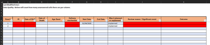
My table, named Input has 11 columns and starts at cell A6 (A6 being the first column header). See attached screenshot.

Above columns, ID / Date of Birth / Delivery mechanism / Review reason / Significant event / Outcome, I would like a count of all the conditionally formatted red cells.

Not sure if it is important, but according to the More Colours section when choosing a colour within the Format.., Red : 255 / Green : 0 / Blue : 0 and the Hex code is #FF0000.

The purpose is to highlight and count the number of missing data.

Thank you in advance!

 

[Automatrix]

I believe you can use the GET.CELL function described here: 6 Ways to Count Colored Cells in Microsoft Excel [Illustrated Guide] | How To Excel

 

[Peter_SSs]

I would like a count of all the conditionally formatted red cells.

What is the condition formatting rule that causes them to be red?
Often, that same rule can be adapted to count them.

 

[_eNVy_]

What is the condition formatting rule that causes them to be red?
Often, that same rule can be adapted to count them.

In the Edit Formatting Rule, Rule Type : Use a formula to determine which cells to format.
The formula used is :

=AND(ISNUMBER(A7),K7="")

A7 is the Row # where if there is any data in any of the cells along the same row, a number will populate.
The formula in this condition is applied similarly to the other columns, all referring to A7 (Row #).

 

[_eNVy_]

I believe you can use the GET.CELL function described here: 6 Ways to Count Colored Cells in Microsoft Excel [Illustrated Guide] | How To Excel

There needs to be a colour count for every column. If I've understood the link you kindly supplied, I would need to have a column for every one of my column headers.
I only wish to have a count above each column header that counts the total number of red cells.

 

[RoryA]

You could use a formula like:

=SUMPRODUCT(ISNUMBER(A7:A100)*(K7:K100<>""))

adjusting the ranges to suit your data.

 

[Peter_SSs]

You could use a formula like:

=SUMPRODUCT(ISNUMBER(A7:A100)*(K7:K100<>""))

To count the red (blank) cells, wouldn't that need to be

=SUMPRODUCT(ISNUMBER(A7:A100)*(B7:B100=""))

@_eNVy_
Since it appears your data is in a formal Excel table you could use something like this then you wouldn't ever have to worry about what number of rows is involved. Adjust the table name if required.

_eNVy_.xlsm
	A	B	C	D	E	F
4		2	1			0
5
6	Row #	ID	Date of Birth	Date of Death	Age Band	Delivery mechanism
7	1					x
8	2		16/08/1986			y
9
10
11
Sheet1

Cell Formulas
Range	Formula
B4	B4	=COUNTIFS(Table1[Row '#],"<>",Table1[ID],"")
C4	C4	=COUNTIFS(Table1[Row '#],"<>",Table1[Date of Birth],"")
F4	F4	=COUNTIFS(Table1[Row '#],"<>",Table1[Delivery mechanism],"")

.. or a variation that you could just drag across the row, and then delete the formula from any columns that you don't want a count for.

_eNVy_.xlsm
	A	B	C	D	E	F
3		2	1			0
5
6	Row #	ID	Date of Birth	Date of Death	Age Band	Delivery mechanism
7	1					x
8	2		16/08/1986			y
9
10
11
Sheet1

Cell Formulas
Range	Formula
B3	B3	=COUNTIFS(Table1[[Row '#]:[Row '#]],"<>",Table1[ID],"")
C3	C3	=COUNTIFS(Table1[[Row '#]:[Row '#]],"<>",Table1[Date of Birth],"")
F3	F3	=COUNTIFS(Table1[[Row '#]:[Row '#]],"<>",Table1[Delivery mechanism],"")

 

[_eNVy_]

You could use a formula like:

=SUMPRODUCT(ISNUMBER(A7:A100)*(K7:K100<>""))

adjusting the ranges to suit your data.

I swapped the

<>""

into

=""

as I needed to count how many blanks there are within the table.
But thank you very much. I was originally trying to incorporate a COUNTIFS and ISNUMBER.
I'm not all that comfortable with SUMPRODUCT.

Again, thank you. This does what I require.

 

[Peter_SSs]

Looks like you are happy with the SUMPRODUCT approach but I wanted to correct my formulas because I forgot that column A actually contains a formula so my previous suggestions will not produce the correct results. Corrected versions of both types of formulas below.

BTW, I suggest that you update your Account details (click your user name at the top right of the forum) so helpers always know what Excel version(s) & platform(s) you are using as the best solution often varies by version. (Don’t forget to scroll down & ‘Save’)

_eNVy_.xlsm
	A	B	C	D	E	F
3		2	1			0
4		2	1			0
5
6	Row #	ID	Date of Birth	Date of Death	Age Band	Delivery mechanism
7	1					x
8	2		16/08/1986			y
9
10
11
Sheet1

Cell Formulas
Range	Formula
B3	B3	=COUNTIFS(Table1[[Row '#]:[Row '#]],">0",Table1[ID],"")
C3	C3	=COUNTIFS(Table1[[Row '#]:[Row '#]],">0",Table1[Date of Birth],"")
B4	B4	=COUNTIFS(Table1[Row '#],">0",Table1[ID],"")
C4	C4	=COUNTIFS(Table1[Row '#],">0",Table1[Date of Birth],"")
F3	F3	=COUNTIFS(Table1[[Row '#]:[Row '#]],">0",Table1[Delivery mechanism],"")
F4	F4	=COUNTIFS(Table1[Row '#],">0",Table1[Delivery mechanism],"")

 

[RoryA]

To count the red (blank) cells, wouldn't that need to be

I was going off the formula in post #4