Count days from date range

[Maride]

I have a list of time off requests that are listed as date ranges (ie. 6/7/21 - 6/10/21 ) and I need to make a count of how many days off are requested for each date, ideally without having to manually input each date between the date ranges. So i want to be able to input


6/7/21 - 6/10/21
6/8/21 - 6/8/21
6/8/21 - 6/9/21
and be able to get a list

6/7/21 - 1
6/8/21 - 3
6/9/21 - 2
6/10/21 1

 

[Joe4]

Welcome to the Board!

The issue is that entries like "6/7/21 - 6/10/21" are text entries, and not date entries. So it is difficult to do mathematical computation on them without creating some conversion formulas instead.

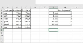
If you have the ability to split up, so you have two columns, one for the Start Date and one for the End Date, this becomes a much easier task.

So let's say that the Start Dates are in A1:A3 and the corresponding end dates are in B1:B3.
And we have the date 6/7/21 in cell A6, and wanted to count how many people have that day off, then we could use this formula:

=COUNTIFS($A$1:$A$3,"<="&A6,$B$1:$B$3,">="&A6)

If you cannot change how you receive the data, and will always receive it like "6/7/21 - 6/10/21", then you can write formulas to split up.
So, for an entry in cell A1, the Start Date formula would look like this:

=DATEVALUE(TRIM(LEFT(SUBSTITUTE(A1,"-",REPT(" ",20)),20)))

and the End Date formula would look like this:

=DATEVALUE(TRIM(RIGHT(SUBSTITUTE(A1,"-",REPT(" ",20)),20)))

 

[Maride]

So I do have them split the issue is howcan i get a count of how many people have 6/8 and 6/9 off if I have 6/7 as start and 6/10 as end without having to manually input a cell for 6/8 and 6/9

 

[Joe4]

So I do have them split the issue is howcan i get a count of how many people have 6/8 and 6/9 off if I have 6/7 as start and 6/10 as end without having to manually input a cell for 6/8 and 6/9

Look again at the first explanation and formula I provided.
That formula returns exactly what you are asking for.

 

[Fluff]

Welcome to the MrExcel Message Board!

Cross-posting (posting the same question in more than one forum) is not against our rules, but the method of doing so is covered by #13 of the Forum Rules.

Be sure to follow & read the link at the end of the rule too!

Cross posted at: Count days off from date range
and Pivot Table from Date Range
If you have posted the question at more places, please provide links to those as well.

If you do cross-post in the future and also provide links, then there shouldn’t be a problem.

 

[Maride]

Look again at the first explanation and formula I provided.
That formula returns exactly what you are asking for.

Maybe Im misunderstanding..I've attached a sample of what I am trying to get

 

[Maride]

Maybe Im misunderstanding..I've attached a sample of what I am trying to get

wait i think it get it..

 

[Maride]

Look again at the first explanation and formula I provided.
That formula returns exactly what you are asking for.

So I have the formula in there its returning a 0 with no errors, but its not returning a count when i list days in that date range

sample.xlsx
	A	B	C	D	E	F	G	H	I
1	Employee	Start Date	End Date				Employees Off
2	Jon	7-Jun	7-Jun			7-Jun	0
3	jack	7-Jun	10-Jun			8-Jun	0
4	sally	9-Jun	10-Jun			9-Jun	0
5	june	10-Jun	10-Jun			10-Jun	0
6	jared	10-Jun	11-Jun			11-Jun	0
7	sue	11-Jun	11-Jun
8
9
Sheet1

Cell Formulas
Range	Formula
G2	G2	=COUNTIFS($B$2:$B$7,"<="&F2,$C$2:$C$7,">=""F2")
G3	G3	=COUNTIFS($B$2:$B$7,"<="&F3,$C$2:$C$7,">=""F3")
G4	G4	=COUNTIFS($B$2:$B$7,"<="&F4,$C$2:$C$7,">=""F4")
G5	G5	=COUNTIFS($B$2:$B$7,"<="&F5,$C$2:$C$7,">=""F5")
G6	G6	=COUNTIFS($B$2:$B$7,"<="&F6,$C$2:$C$7,">=""F6")

 

[Joe4]

You have a typo in your formula. You have a bunch of quotes around the last range reference, which then makes it the literal text value "F2", not the cell D2.
Try changing the formula in G2 to:
=COUNTIFS($B$2:$B$7,"<="&F2,$C$2:$C$7,">=" & F2)

 

[Maride]

You have a typo in your formula. You have a bunch of quotes around the last range reference, which then makes it the literal text value "F2", not the cell D2.
Try changing the formula in G2 to:
=COUNTIFS($B$2:$B$7,"<="&F2,$C$2:$C$7,">=" & F2)

OMG IT WORKED thank you so much!