Count distinct text values from column with specific conditions within that cell

[Fishboy]

Hi guys, long time no post!

I am currently helping someone who is using Excel to outline the schedule for multiple users across a month, and then using this to count and track workload and types of jobs carried out.

KEY POINT - I Cannot use any VBA solutions as macro enabled workbooks are not allowed

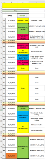
As per the attached image, columns A and B cover the dates throughout the month going downwards.

Column C shows the tester's schedule. An engagement which lasts more than one day has been merged into a single cell (I know, merged cells are a nightmare!)

Column E is a helper column which is usually hidden, but effectively it works out the value of the adjacent cell for counting purposes as the merged cells otherwise only count as 1. Dont think they will be useful for this task, but they are there if needed and I use them for a separate counting function anyways.

I need to be able to count the distinct values from either column C or E. Basically I am being asked to count how many distinct instances there are of cells containing (LHE), (LFE) or (SFE) within them, separated into the ones which also contain "Testing" or "CE Plus". They need to be distinct as sometimes (as per the example) "MEMBER 1 Testing (R) (LHE)" occurs more than once in the month and should only be counted once.

I had been using variations of the following formula depending on what I was counting, but these count the duplicates as well.
=COUNTIFS($C$6:$C$36,"*Testing*",$C$6:$C$36,"*(LFE)*")

I had also tried using this to count the distinct values, but I have not found a way to incorporate the additional conditions for "Testing" and the (LHE) criteria for example
{=SUM(IF(LEN(E6:E36),1/COUNTIF(E6:E36,E6:E36)))}

Can anyone offer any suggestions that may assist, or am I just making things too complicated?

Thanks in advance,

Fishboy!

 

[DanteAmor]

How about:

Dante Amor
	A	B	C	D	E	F	G
1
5							Result
6		01-mar	member 1 testing (R) (LHE)		Testing	(LHE)	1
7		02-mar	ce plus read test member (LFE)		Testing	(LFE)	1
8		03-mar	member 1 testing (R) (LHE)		Testing	(SFE)	0
9		04-mar	iso documentation		CE Plus	(LHE)	0
10		05-mar	member 1 testing (R) (LHE)		CE Plus	(LFE)	1
11		06-mar	member 1 testing (R) (LHE)		CE Plus	(SFE)	0
12		07-mar	ce plus read testing member (LFE)
13		08-mar	member 1 testing (R) (LHE)
14		09-mar	ce plus read testing member (LFE)
15		10-mar	member 1 testing (R) (LHE)
16
Hoja1

Cell Formulas
Range	Formula
G6:G11	G6	=IFERROR(IF(MATCH("*"&E6&"*"&F6&"*",$C$6:$C$20,0),1),0)

 

[Fishboy]

Hi Dante, that seems to work just great! Totally different approach than I had even considered!

Thanks!

 

[DanteAmor]

I'm glad to help you. Thanks for the feedback.

 

[Fishboy]

I'm glad to help you. Thanks for the feedback.

Hi again Dante,

I was wondering whether this could be expanded at all. Effectively the example I gave is for a single tester within my workbook, but basically the tester column is mirrored a number of times across the sheet for each additional tester (the columns specifically to be looked in are every 3rd column starting at column C). Would it be possible to include the width of the table as well as the length of the column to count for unique values?

I am currently using this amended version of your formula so it adds the count for each of the testers:

=IFERROR(IF(MATCH("*Testing*"&"*LFE*",$C$6:$C$35,0),1),0)+IFERROR(IF(MATCH("*Testing*"&"*LFE*",$F$6:$F$35,0),1),0)+IFERROR(IF(MATCH("*Testing*"&"*LFE*",$I$6:$I$35,0),1),0)+IFERROR(IF(MATCH("*Testing*"&"*LFE*",$L$6:$L$35,0),1),0)+IFERROR(IF(MATCH("*Testing*"&"*LFE*",$O$6:$O$35,0),1),0)+IFERROR(IF(MATCH("*Testing*"&"*LFE*",$R$6:$R$35,0),1),0)+IFERROR(IF(MATCH("*Testing*"&"*LFE*",$U$6:$U$35,0),1),0)+IFERROR(IF(MATCH("*Testing*"&"*LFE*",$X$6:$X$35,0),1),0)+IFERROR(IF(MATCH("*Testing*"&"*LFE*",$AA$6:$AA$35,0),1),0)+IFERROR(IF(MATCH("*Testing*"&"*LFE*",$AD$6:$AD$35,0),1),0)+IFERROR(IF(MATCH("*Testing*"&"*LFE*",$AG$6:$AG$35,0),1),0)+IFERROR(IF(MATCH("*Testing*"&"*LFE*",$AJ$6:$AJ$35,0),1),0)+IFERROR(IF(MATCH("*Testing*"&"*LFE*",$AM$6:$AM$35,0),1),0)

Ideally if I could get a singular formula rather than a doctored one with lots of +the same formula again that would be most helpful. The dimensions of the range would be from C6 to AM35.

I tried amending your formula to this but it returned a zero value which I know to be wrong:

=IFERROR(IF(MATCH("*Pen Test*"&"*LFE*",$C$6:$AM$35,0),1),0)

Thanks again for your help.

 

[DanteAmor]

Sorry for taking a while to answer, I'm busy with my work, hehe.
Try this:

Dante Amor
	A	B	C	D	E	F	G	H	I
1
5					1
6		01-mar	member 1 testing (R) (LHE)			member 1 testing (R) (LHE)			member 1 testing (R) (LHE)
7		02-mar	ce plus read test member (LFE)			ce plus read test member (LFE)			ce plus read test member (LxE)
8		03-mar	member 1 testing (R) (LHE)			member 1 testing (R) (LHE)			member 1 testing (R) (LyE)
9		04-mar	iso documentation			iso documentation			iso documentation
10		05-mar	member 1 testing (R) (LHE)			member 1 testing (R) (LHE)			member 1 testing (R) (LHE)
11		06-mar	member 1 testing (R) (LHE)			member 1 testing (R) (LHE)			member 1 testing (R) (LHE)
12		07-mar	ce plus read testing member (LFE)			ce plus read testing member (LFE)			ce plus read testing member (LFE)
13		08-mar	member 1 testing (R) (LHE)			member 1 testing (R) (LHE)			member 1 testing (R) (LHE)
14		09-mar	ce plus read testing member (LFE)			ce plus read testing member (LFE)			ce plus read testing member (LFE)
15		10-mar	member 1 testing (R) (LHE)			member 1 testing (R) (LHE)			member 1 testing (R) (LHE)
Hoja1b

Cell Formulas
Range	Formula
E5	E5	=IF(SUM(--ISNUMBER(SEARCH("*testing*LHE*",C6:AM15)))>0,1,0)
Press CTRL+SHIFT+ENTER to enter array formulas.

 

[Fishboy]

Hi Dante, thanks for your reply, and don't worry about the delay

Unfortunately, while this does work in your example, it doesn't work in situ in my workbook. Plus, after a little experimentation with your example dataset I am not sure it is quite doing what I need it to.

Let's say you change the value in C6 so it says member 2 instead of member 1, but the rest remains unchanged. What I would hope for it that the count would raise from 1 to 2, as there will now be 2 distinctly different entries that contain both "testing" and *LHE* across the table.

Does this make sense?

 

[DanteAmor]

If all the texts to consider have the text "member" and the member number is unique, then it could be something like this.
Change the number 20 to the number of members ($1:$20)

Dante Amor
	A	B	C	D	E	F	G	H	I	J	K	L
1
2
3		Testing-LFE	2
4		Testing-SFE	3
5
6		01-mar	member 1 testing (R) (LFE)			member 8 testing (SFE)			member 9 testing (SFE)			member 6 testing (SFE)
7		02-mar	member 6 testing (SFE)			member 1 testing (R) (LFE)			member 9 testing (SFE)			member 8 testing (SFE)
8		03-mar	member 6 testing (SFE)			member 8 testing (SFE)			member 9 testing (SFE)			member 9 testing (SFE)
9		04-mar	member 6 testing (SFE)			member 8 testing (SFE)			member 9 testing (SFE)			member 1 testing (R) (LFE)
10		05-mar	member 6 testing (SFE)			member 8 testing (SFE)			member 9 testing (SFE)			member 6 testing (SFE)
11		06-mar	member 6 testing (SFE)			member 2 testing (R) (LFE)			member 9 testing (SFE)			member 8 testing (SFE)
12		07-mar	member 1 testing (R) (LFE)			member 8 testing (SFE)			member 9 testing (SFE)			member 9 testing (SFE)
13		08-mar	member 6 testing (SFE)			member 8 testing (SFE)			member 9 testing (SFE)			member 6 testing (SFE)
14		09-mar	member 6 testing (SFE)			member 8 testing (SFE)			member 9 testing (SFE)			member 8 testing (SFE)
15		10-mar	member 6 testing (SFE)			member 1 testing (R) (LFE)			member 2 testing (R) (LFE)			member 9 testing (SFE)
Hoja1b

Cell Formulas
Range	Formula
C3	C3	=SUM(--(FREQUENCY(IF(ISNUMBER(SEARCH("*testing*LFE*",$C$6:$L$15)),LEFT(SUBSTITUTE(MID($C$6:$L$15,SEARCH("member",$C$6:$L$15)+7,LEN($C$6:$L$15))," ",REPT(" ",99)),99)+0),ROW($1:$20))>0))
C4	C4	=SUM(--(FREQUENCY(IF(ISNUMBER(SEARCH("*testing*SFE*",$C$6:$L$15)),LEFT(SUBSTITUTE(MID($C$6:$L$15,SEARCH("member",$C$6:$L$15)+7,LEN($C$6:$L$15))," ",REPT(" ",99)),99)+0),ROW($1:$20))>0))
Press CTRL+SHIFT+ENTER to enter array formulas.

 

[Fishboy]

Hi Dante, I think I may have oversimplified my example data too much and as a result this will not work either. The cells will contain the following information:

1. Member name (The name of a company from a massive list of 400+ entities)
2. Testing
3. A category from (LHE), (LFE) or (SFE)

It will be the specific member name that is the unique identifier, as multiple cells could contain the exact same data for information points 2 and 3. Unfortunately the actual name of the member is dynamic and could be anything really, but this is what I need to check for and count the unique instances that also include points 2 and 3.

 

[DanteAmor]

You could give a representative example of your data, use XL2BB tool minisheet. There you must also show the results you want.