Count of # SKUs it takes to get to 80% of the sales for a specific criteria

[HollyBB]

Hello. Newbie here. I need help with I think may be a very simple formula that I can not get my head around. I've tried match, sumproduct, countif(s) ... you name it! I've spent the last 2 days searching the internet & find "close" solutions, but not one that will work for me. I have a spreadsheet with about 3000 rows. The spreadsheet is sorted by total sales in descending order. Col A contains 3000 SKU#s. Each SKU # belongs to 1 of 20 distinct "classes". I'm trying to create a formula at the "class" level. I have the 20 distinct classes listed in Col D.
I calculated the sum of sales by distinct class in Col E. Then I calculated 80% of those sales in Col F.
What I need is a formula in Col G that says (for example): How many SKUs does it take (count) to get the "closest" to 80% of their class sales. The # of SKUs can result in > or < 80%- just needs to be the closest.
For example, how many SKUs (rows?) in class 943 does it take to sum to (close to) 10,305,237? Summing from top to bottom of row F?
Any help would be much appreciated And of course it was due "yesterday"

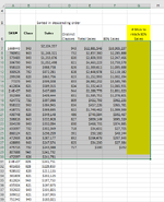
Col A Col B Col C Col D Col E Col F Col G
1. SKU# Class Sales Distinct Class Total Sales 80% of Sales # SKUs to get to 80% of sales
2. 1668443 943 $2,104,337 943 $12,881,546 $10,305,237 ?
3. 760951 943 $1,246,321 732 $2,857,360 $2,285,888 ?
4. 573483 943 $1,213,076 820 $2,809,333 $2,247,466 ?
5. 506790 943 $1,052,498 821 $4,663,223 $3,730,578 ?
6. 958103 943 $988,738 826 $1,369,611 $1,095,688 ?
7. 300525 732 $972,281 828 $2,648,978 $2,119,182 ?

 

[JamesCanale]

I had to pop out of dynamic array size matching at the end and resort to iferror(xxx,""). I hate when that happens. I'll be interested if fluff can fix it.

MrExcelPlayground15.xlsx
	A	B	C	D	E	F	G
2	SKU	Class	Sales	Distinct Classes	Total Sales	80%	# SKUS to reach 80%
3	4650	943	$2,100,000	943	$21,483,223	$17,186,578	10
4	1498	943	$2,011,236	732	$5,800,202	$4,640,162	3
5	4644	943	$1,996,827	820	$4,293,616	$3,434,893	2
6	8369	943	$1,906,509	821	$7,492,032	$5,993,625	4
7	3341	943	$1,893,101	826	$5,419,367	$4,335,494	4
8	3034	732	$1,885,222	828	$1,172,189	$937,751	1
9	8143	820	$1,880,716
10	2758	943	$1,830,752
11	9052	821	$1,813,968
12	8446	943	$1,812,024
13	4900	821	$1,732,512
14	3193	732	$1,644,815
15	6470	943	$1,577,623
16	8875	821	$1,478,944
17	4978	820	$1,382,242
18	1621	943	$1,315,552
19	8286	943	$1,249,300
20	9954	732	$1,183,279
21	6626	821	$1,181,805
22	3329	826	$1,108,543
23	9888	943	$1,107,104
24	6122	732	$1,086,886
25	7201	943	$1,080,239
26	4638	826	$1,045,946
27	4353	826	$1,028,388
28	6563	826	$936,418
29	1169	828	$849,867
30	4565	820	$763,270
31	5829	943	$670,779
32	3455	821	$629,542
33	1056	943	$626,775
34	8909	821	$529,394
35	3550	826	$462,337
36	3262	826	$419,264
37	2742	826	$418,471
38	8836	828	$322,322
39	7978	820	$267,387
40	3736	943	$212,020
41	4369	821	$125,867
42	6815	943	$93,384
Sheet2

Cell Formulas
Range	Formula
D3:D8	D3	=UNIQUE(B3:B42)
E3:E8	E3	=SUMIF($B$3:$B$42,D3#,$C$3:$C$42)
F3:F8	F3	=0.8*E3#
G3:G21	G3	=IFERROR(LET(a,FILTER($C$3:$C$42,$B$3:$B$42=D3),b,SEQUENCE(ROWS(a),ROWS(a)),c,IF(MOD(b-1,ROWS(a))+1>=INT((b-1)/ROWS(a))+1,1,0),d,MMULT(SEQUENCE(1,ROWS(a),1,0),c*a),e,ABS(d-F3),MATCH(MIN(e),e,0)),"")
Dynamic array formulas.

 

[HollyBB]

Thank You for your response. I only encountered 1 issue: I'm running out of resources (there are actually 6k rows). Any other work-around?

 

[HollyBB]

16k rows

 

[JamesCanale]

The arrays made must get too big. 3000 records is too many for it.

 

[JamesCanale]

New helper column in D:

MrExcelPlayground15.xlsx
	A	B	C	D	E	F	G	H
2	SKU	Class	Sales	running class	Distinct Classes	Total Sales	80%	# SKUS to reach 80%
3	4650	943	$2,100,000	$2,100,000	943	$21,483,223	$17,186,578	10
4	1498	943	$2,011,236	$4,111,236	732	$5,800,202	$4,640,162	3
5	4644	943	$1,996,827	$6,108,063	820	$4,293,616	$3,434,893	2
6	8369	943	$1,906,509	$8,014,572	821	$7,492,032	$5,993,625	4
7	3341	943	$1,893,101	$9,907,672	826	$5,419,367	$4,335,494	4
8	3034	732	$1,885,222	$1,885,222	828	$1,172,189	$937,751	1
9	8143	820	$1,880,716	$1,880,716
10	2758	943	$1,830,752	$11,738,424
11	9052	821	$1,813,968	$1,813,968
12	8446	943	$1,812,024	$13,550,448
13	4900	821	$1,732,512	$3,546,480
14	3193	732	$1,644,815	$3,530,037
15	6470	943	$1,577,623	$15,128,071
16	8875	821	$1,478,944	$5,025,424
17	4978	820	$1,382,242	$3,262,959
18	1621	943	$1,315,552	$16,443,623
19	8286	943	$1,249,300	$17,692,923
20	9954	732	$1,183,279	$4,713,316
21	6626	821	$1,181,805	$6,207,229
22	3329	826	$1,108,543	$1,108,543
23	9888	943	$1,107,104	$18,800,027
24	6122	732	$1,086,886	$5,800,202
25	7201	943	$1,080,239	$19,880,266
26	4638	826	$1,045,946	$2,154,489
27	4353	826	$1,028,388	$3,182,877
28	6563	826	$936,418	$4,119,295
29	1169	828	$849,867	$849,867
30	4565	820	$763,270	$4,026,229
31	5829	943	$670,779	$20,551,045
32	3455	821	$629,542	$6,836,771
33	1056	943	$626,775	$21,177,819
34	8909	821	$529,394	$7,366,165
35	3550	826	$462,337	$4,581,632
36	3262	826	$419,264	$5,000,896
37	2742	826	$418,471	$5,419,367
38	8836	828	$322,322	$1,172,189
39	7978	820	$267,387	$4,293,616
40	3736	943	$212,020	$21,389,839
41	4369	821	$125,867	$7,492,032
42	6815	943	$93,384	$21,483,223
Sheet2

Cell Formulas
Range	Formula
E3:E8	E3	=UNIQUE(B3:B42)
F3:F8	F3	=SUMIF($B$3:$B$42,E3#,$C$3:$C$42)
G3:G8	G3	=0.8*F3#
H3:H8	H3	=MATCH(MIN(ABS(FILTER($D$3:$D$42,$B$3:$B$42=E3)-G3)),ABS(FILTER($D$3:$D$42,$B$3:$B$42=E3)-G3),0)
D3:D42	D3	=SUMIF(B$3:B3,B3,C$3:C3)
Dynamic array formulas.

 

[Fluff]

How about

Fluff.xlsm
	A	B	C	D	E	F	G
1
2	SKU	Class	Sales	Distinct Classes	Total Sales	0.8	# SKUS to reach 80%
3	4650	943	2100000	943	21483223	17186578	10
4	1498	943	2011236	732	5800202	4640162	3
5	4644	943	1996827	820	4293616	3434893	2
6	8369	943	1906509	821	7492032	5993625	4
7	3341	943	1893101	826	5419367	4335494	4
8	3034	732	1885222	828	1172189	937750.9	1
9	8143	820	1880716
10	2758	943	1830752
11	9052	821	1813968
12	8446	943	1812024
13	4900	821	1732512
14	3193	732	1644815
15	6470	943	1577623
16	8875	821	1478944
17	4978	820	1382242
18	1621	943	1315552
19	8286	943	1249300
20	9954	732	1183279
21	6626	821	1181805
22	3329	826	1108543
23	9888	943	1107104
24	6122	732	1086886
25	7201	943	1080239
26	4638	826	1045946
27	4353	826	1028388
28	6563	826	936418.2
29	1169	828	849866.5
30	4565	820	763270.4
31	5829	943	670778.7
32	3455	821	629542
33	1056	943	626774.6
34	8909	821	529393.9
35	3550	826	462336.5
36	3262	826	419264.4
37	2742	826	418471.3
38	8836	828	322322.1
39	7978	820	267386.7
40	3736	943	212019.8
41	4369	821	125867.2
42	6815	943	93383.52
Main

Cell Formulas
Range	Formula
D3:D8	D3	=UNIQUE(B3:B42)
E3:E8	E3	=SUMIF($B$3:$B$42,D3#,$C$3:$C$42)
F3:F8	F3	=0.8*E3#
G3:G8	G3	=LET(s,SCAN(0,FILTER($C$3:$C$100,$B$3:$B$100=D3),LAMBDA(x,y,x+y)),XMATCH(MIN(ABS(F3-s)),ABS(F3-s),0))
Dynamic array formulas.

 

[Fluff]

Another option that will spill down in col G

=DROP(REDUCE("",SEQUENCE(ROWS(D3#)),LAMBDA(a,b,LET(s,SCAN(0,FILTER($C$3:$C$100,$B$3:$B$100=INDEX(D3#,b)),LAMBDA(x,y,x+y)),VSTACK(a,XMATCH(MIN(ABS(INDEX(F3#,b)-s)),ABS(INDEX(F3#,b)-s),0))))),1)

 

[HollyBB]

How about

Thank You SOOOOO much This works GREAT! Could I add one more criteria to the question. If I added an additional column (H) which contained the words either "Active" or "Inactive", could you adjust your existing formula to only look at the "Active" SKUs? (ignore those rows that contained "Inactive" in column H ????

 

[Fluff]

Can you post some sample data.

MrExcel has a tool called “XL2BB” that lets you post samples of your data that will allow us to copy/paste it to our Excel spreadsheets, so we can work with the same copy of data that you are. Instructions on using this tool can be found here: XL2BB Add-in

Note that there is also a "Test Here” forum on this board. This is a place where you can test using this tool (or any other posting techniques that you want to test) before trying to use those tools in your actual posts.