Count the data in column on sheet 2 from results in column on sheet 1 after matching data in corresponding column

[DanJones]

Sheet1

Sheet 2

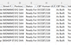
Hi, I am trying to do a calculation if column D in Sheet 1 = As Built, it takes the corresponding data in Column K and counts the occurrences of it in Column H on Sheet 2. I have tried all sorts of combinations of INDEX, COUNT, SUMPRODUCT etc. the closest I am getting is =SUMPRODUCT(--ISNUMBER(MATCH('CBT OR Chamber'!K:K,'SY-property-statuses'!H:H,0))) but that is not taking into account the column D in Sheet 1 = As Built. Please help, new to this forum and it's the first time I have been this stuck, so sorry if it is a stupid repeated question!

 

[Fluff]

Hi & welcome to MrExcel.
Which sheet are you putting the formula in?

 

[DanJones]

Thank you, I am putting the formula in a separate summary sheet

 

[Fluff]

Ok, how about

=ROWS(FILTER('SY-property-statuses'!H2:H1000,ISNUMBER(MATCH('SY-property-statuses'!H2:H1000,FILTER('CBT OR Chamber'!K2:K1000,'CBT OR Chamber'!D2:D1000="As Built"),0))))

 

[DanJones]

I am getting #CALC! ... I think because some of the cells in sheet 2 column H are blank, is there a quick way to ignore blanks or have I misunderstood the result.

 

[Fluff]

The #Calc means that one of the two filter functions returned no results.
If you use this, does it return anything

=FILTER('CBT OR Chamber'!K2:K1000,'CBT OR Chamber'!D2:D1000="As Built")

 

[DanJones]

That gives me #SPILL! I do not have "As Built" in column K, only in column D, in column K I have a list as shown above, it is the corresponding data next to "As Built" i.e. in the example above SY/CBT/159 that I want to count the occurrences of it in Column H on Sheet 2, SY/CBT/159 would be 10 but in the example above I would want the total of SY/CBT/159, SY/CBT/160, SY/CBT/161 up to SY/CBT/164

 

[Fluff]

That gives me #SPILL!

That means that it has found some values, but there are populated cells stopping the formula from spilling down.
Which suggests that the values from col K where not found in col H on the other sheet.

 

[DanJones]

Odd, it is as you can see above the values from col K are shown in col H in the 2 examples above with the example I have given - SY/CBT/159

 

[Fluff]

Check that none of those values have leading/trailing spaces, or other hidden characters.