Hello Excel wizards! I have attempted about a dozen formulas to get the outcome I need and I fall short each time! I'm certain this will be a piece of cake for you!
I have tried to paste in the "mini sheet" to make it easy to help. Fingers Crossed.
There are two tabs- "Metrics Review" tab lists activities horizontally across a time span (with date name titles I can't change as they are consistent with a larger data in the spreadsheet) and "Milestones" tab which is a linked data set from a power pivot that I need to use in my formula.
Here is the calculation I need help with-
On "Milestones" Count the # of occurrences from the pivot given the project #, month, and year. On the "Metrics Review" Subtract the recorded closings for the matching project/month/year from that Milestones count, but return zero if the month is in the past, and return zero if the month is both in the future AND not represented on the pivot.
So for example
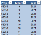
Power Pivot tab "Milestones"
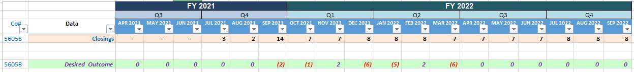
Timeline tab "Metrics Review"
I have tried to paste in the "mini sheet" to make it easy to help. Fingers Crossed.
There are two tabs- "Metrics Review" tab lists activities horizontally across a time span (with date name titles I can't change as they are consistent with a larger data in the spreadsheet) and "Milestones" tab which is a linked data set from a power pivot that I need to use in my formula.
Here is the calculation I need help with-
On "Milestones" Count the # of occurrences from the pivot given the project #, month, and year. On the "Metrics Review" Subtract the recorded closings for the matching project/month/year from that Milestones count, but return zero if the month is in the past, and return zero if the month is both in the future AND not represented on the pivot.
So for example
- September 2021 there are 12 occurrences on the pivot and subtracting the 14 closings returns the value of 14.
- April 2022 there are no occurrences on the pivot so it should just stop and be zero without trying to subtract the seven closings.
Power Pivot tab "Milestones"
| count help 092121.xlsm | |||||
|---|---|---|---|---|---|
| A | B | C | |||
| 3 | Project2 | Month | Year | ||
| 4 | 56058 | 9 | 2021 | ||
| 5 | 56058 | 9 | 2021 | ||
| 6 | 56058 | 9 | 2021 | ||
| 7 | 56058 | 9 | 2021 | ||
| 8 | 56058 | 10 | 2021 | ||
| 9 | 56058 | 10 | 2021 | ||
| 10 | 56058 | 10 | 2021 | ||
| 11 | 56058 | 11 | 2021 | ||
| 12 | 56058 | 10 | 2021 | ||
| 13 | 56058 | 10 | 2021 | ||
| 14 | 56058 | 11 | 2021 | ||
| 15 | 56058 | 11 | 2021 | ||
| 16 | 56058 | 10 | 2021 | ||
| 17 | 56058 | 2 | 2022 | ||
| 18 | 56058 | 2 | 2022 | ||
| 19 | 56058 | 2 | 2022 | ||
| 20 | 56058 | 3 | 2022 | ||
| 21 | 56058 | 2 | 2022 | ||
| 22 | 56058 | 2 | 2022 | ||
| 23 | 56058 | 2 | 2022 | ||
| 24 | 56058 | 2 | 2022 | ||
| 25 | 56058 | 2 | 2022 | ||
| 26 | 56058 | 2 | 2022 | ||
| 27 | 56058 | 2 | 2022 | ||
| 28 | 56058 | 1 | 2022 | ||
| 29 | 56058 | 1 | 2022 | ||
| 30 | 56058 | 1 | 2022 | ||
| 31 | 56058 | 12 | 2021 | ||
| 32 | 56058 | 11 | 2021 | ||
| 33 | 56058 | 11 | 2021 | ||
| 34 | 56058 | 11 | 2021 | ||
| 35 | 56058 | 12 | 2021 | ||
| 36 | 56058 | 11 | 2021 | ||
| 37 | 56058 | 11 | 2021 | ||
| 38 | 56058 | 11 | 2021 | ||
| 39 | 56058 | 9 | 2021 | ||
| 40 | 56058 | 9 | 2021 | ||
| 41 | 56058 | 9 | 2021 | ||
| 42 | 56058 | 9 | 2021 | ||
| 43 | 56058 | 9 | 2021 | ||
| 44 | 56058 | 9 | 2021 | ||
| 45 | 56058 | 9 | 2021 | ||
| 46 | 56058 | 9 | 2021 | ||
| 47 | 56058 | 1 | 1900 | ||
| 48 | 56058 | 1 | 1900 | ||
Milestones | |||||
Timeline tab "Metrics Review"
| count help 092121.xlsm | |||||||||||||||||||||||||||||
|---|---|---|---|---|---|---|---|---|---|---|---|---|---|---|---|---|---|---|---|---|---|---|---|---|---|---|---|---|---|
| A | B | J | K | L | M | N | O | P | Q | R | S | T | U | V | W | X | Y | Z | AA | ||||||||||
| 4 | Q3 | Q4 | Q1 | Q2 | Q3 | Q4 | |||||||||||||||||||||||
| 5 | Co# | Data | APR 2021 | MAY 2021 | JUN 2021 | JUL 2021 | AUG 2021 | SEP 2021 | OCT 2021 | NOV 2021 | DEC 2021 | JAN 2022 | FEB 2022 | MAR 2022 | APR 2022 | MAY 2022 | JUN 2022 | JUL 2022 | AUG 2022 | SEP 2022 | |||||||||
| 6 | 56058 | Closings | - | - | - | 3 | 2 | 14 | 7 | 7 | 8 | 8 | 8 | 7 | 7 | 7 | 7 | 8 | 8 | 8 | |||||||||
| 7 | |||||||||||||||||||||||||||||
| 8 | |||||||||||||||||||||||||||||
| 9 | 56058 | Desired Outcome | 0 | 0 | 0 | 0 | 0 | (2) | (1) | 2 | (6) | (5) | 2 | (6) | 0 | 0 | 0 | 0 | 0 | 0 | |||||||||
Metrics Review | |||||||||||||||||||||||||||||
| Cell Formulas | ||
|---|---|---|
| Range | Formula | |
| O9 | O9 | =12-O6 |
| P9 | P9 | =6-P6 |
| Q9 | Q9 | =9-Q6 |
| R9 | R9 | =2-R6 |
| S9 | S9 | =3-S6 |
| T9 | T9 | =10-T6 |
| U9 | U9 | =1-U6 |
| Cells with Conditional Formatting | ||||
|---|---|---|---|---|
| Cell | Condition | Cell Format | Stop If True | |
| D6:O8 | Cell Value | <0 | text | NO |