Hello all,
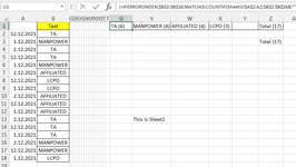
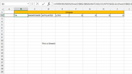
I am looking to count specific text when filtered. I am having the hardest time trying to piece the formula together. I have attached a link to of my example.
I am looking to count specific text when filtered. I am having the hardest time trying to piece the formula together. I have attached a link to of my example.
| Countif ssubtotal.xlsx | |||||||||||||||||||||||||||
|---|---|---|---|---|---|---|---|---|---|---|---|---|---|---|---|---|---|---|---|---|---|---|---|---|---|---|---|
| A | B | C | D | E | F | G | H | I | J | K | L | M | N | O | P | Q | R | S | T | U | V | W | X | Y | |||
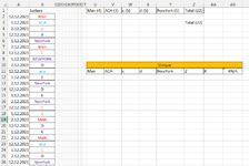
| 2 | A (5) | B (5) | C (5) | Total (15) | E (5) | ||||||||||||||||||||||
| 3 | 12-Dec-21 | a | WHEN I FILTER I WOULD LIKE EACH ONE OF THESE NUMBERS TO CHANGE WITH SUBTOTAL FORMULA | ||||||||||||||||||||||||
| 4 | 12-Jan-21 | b | |||||||||||||||||||||||||
| 5 | 12-Feb-21 | c | |||||||||||||||||||||||||
| 6 | 12-Dec-21 | d | |||||||||||||||||||||||||
| 7 | 12-Jan-21 | e | |||||||||||||||||||||||||
| 8 | 12-Feb-21 | A | |||||||||||||||||||||||||
| 9 | 12-Dec-21 | C | |||||||||||||||||||||||||
| 10 | 12-Jan-21 | E | |||||||||||||||||||||||||
| 11 | 12-Feb-21 | D | |||||||||||||||||||||||||
| 12 | 12-Dec-21 | B | |||||||||||||||||||||||||
| 13 | 12-Jan-21 | A | |||||||||||||||||||||||||
| 14 | 12-Feb-21 | E | |||||||||||||||||||||||||
| 15 | 12-Dec-21 | D | |||||||||||||||||||||||||
| 16 | 12-Jan-21 | B | |||||||||||||||||||||||||
| 17 | 12-Feb-21 | E | |||||||||||||||||||||||||
| 18 | 12-Dec-21 | C | |||||||||||||||||||||||||
| 19 | 12-Jan-21 | C | |||||||||||||||||||||||||
| 20 | 12-Feb-21 | A | |||||||||||||||||||||||||
| 21 | 12-Dec-21 | D | |||||||||||||||||||||||||
| 22 | 12-Jan-21 | B | |||||||||||||||||||||||||
| 23 | 12-Feb-21 | A | |||||||||||||||||||||||||
| 24 | 12-Dec-21 | B | |||||||||||||||||||||||||
| 25 | 12-Jan-21 | C | |||||||||||||||||||||||||
| 26 | 12-Feb-21 | D | |||||||||||||||||||||||||
| 27 | 12-Dec-21 | E | |||||||||||||||||||||||||
| 28 | |||||||||||||||||||||||||||
Sheet1 | |||||||||||||||||||||||||||
| Cell Formulas | ||
|---|---|---|
| Range | Formula | |
| U2 | U2 | ="A ("&COUNTIF($Q$3:$Q$27,"a")&")" |
| V2 | V2 | ="B ("&COUNTIF($Q$3:$Q$27,"B")&")" |
| W2 | W2 | ="C ("&COUNTIF($Q$3:$Q$27,"C")&")" |
| X2 | X2 | ="Total ("&SUM(COUNTIF($Q$3:$Q$27,"a"),COUNTIF($Q$3:$Q$27,"b"),COUNTIF($Q$3:$Q$27,"c"))&")" |
| Y2 | Y2 | ="E ("&COUNTIF($Q$3:$Q$27,"E")&")" |