Counting consecutive Zeros

[RandyD123]

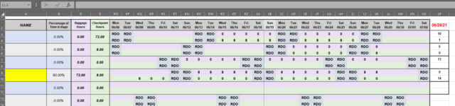
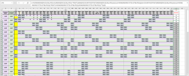
I am trying to count consecutive Zeros on each row. This would have to exclude "RDO". My range starts at F3. The count would be on today's date in column "LP". All rows have data validation that only allows whole numbers 1-10 in quarter hour increments or RDO. If any cell in the row gets a number the count would have to start over. Once the count reaches 14 consecutive zero's the name would highlight in yellow. If the count gets broken after 14 by a number then the count starts over. I have a sheet posted here. I'm not sure if this would be a macro or a formula. Any help would be much appreciated. Thanks

 

[kvsrinivasamurthy]

Upload an example in the file. Explain with example what is required.

 

[RandyD123]

Upload an example in the file. Explain with example what is required.

I did. the link is in the post

 

[RandyD123]

I should also say that the anytime a number is put in the row, other than zero the count starts over. Example would be that you have a 0, 0, RDO, RDO, 0, 0 ......a 4 needs to show in "LP" If it goes like 0, RDO, RDO, 3....then the "LP" column would show 0. But it would have show a 1 on the first day and stayed at 1 on day 2 and day 3, then reset to 0 on day 4.

 

[RandyD123]

More Info:

What I need is a formula that will work in column LP for each row.

Info that may help:

Each person has two rows because they can be in 1 of 2 location each day. Some days they may spend a few hours in each location.

My range is from F3 to LO3 for each person. All columns below row 2 are manual entries, except column LP!!

I only need to track consecutive zeros but not include RDO's

The date in the LP column will change to todays date using =TODAY()

Once any row for a person hits 14, meaning 14 consecutive zero's, not including RDO's their name has to change to yellow.

If a person gets any number on any given day, other than zero or RDO the count has to start over. Basically RDO's should be completely ignored, and only zero's get counted

In the example you can see what it should look like and what should happen.

On 6/29 column LL will get a manual input of either a whole number in quarter hour increments or get a zero or get another RDO.

LP3 counted 10 consecutive zero's and on 6/29 if they get a any number other than zero that current value of 10 has to change to a 0. If they get a zero on 6/29 that current value of 10 has to change to 11

LP4 counted 1 zero and on 6/29 it will either change to a 2 or if they get a number it has to change to 0

LP7 has to change to either 0 or 14, depending on what gets entered on 6/29. If it changes to 14 their name has to highlight in yellow.

LP10 has a 14 which means that their name should have highlighted in yellow on 6/28. If they get a number on 6/29, that value of 14 has to change to 0 and their name will lose the highlight.

I have a sheet on GDrive. Any help would be very much appreciated. Thank You.

 

[kvsrinivasamurthy]

In LP3 then copied down. It is an ARRAY formula. In the image LP2 value I have changed for verification. Helper cell LP1 is used.

=IF(OR(INDEX($F3:$LO3,LP$1)=0,INDEX($F3:$LO3,LP$1)="RDO"),MAX(IF(COUNTIF(OFFSET(INDEX($F3:$LO3,LP$1),0,0,1,0-ROW(INDIRECT("$1:$"&LP$1))),0)+COUNTIF(OFFSET(INDEX($F3:$LO3,LP$1),0,0,1,0-ROW(INDIRECT("$1:$"&LP$1))),"RDO")=ROW(INDIRECT("$1:$"&LP$1)),ROW(INDIRECT("$1:$"&LP$1)),"")),0)

In Helper cell LP1

=INDEX(COLUMN($F$2:$LO$2),MATCH($LP2,$F$2:$LO$2,0))-COLUMN($E$1)

To enter ARRAY formula
Copy and paste the formula in cell
Press F2
Press Ctrl+Shift+Enter together
Excel covers the formula with {}.

 

[RandyD123]

It looks like it is counting RDO's.

In LP3 then copied down. It is an ARRAY formula. In the image LP2 value I have changed for verification. Helper cell LP1 is used.

=IF(OR(INDEX($F3:$LO3,LP$1)=0,INDEX($F3:$LO3,LP$1)="RDO"),MAX(IF(COUNTIF(OFFSET(INDEX($F3:$LO3,LP$1),0,0,1,0-ROW(INDIRECT("$1:$"&LP$1))),0)+COUNTIF(OFFSET(INDEX($F3:$LO3,LP$1),0,0,1,0-ROW(INDIRECT("$1:$"&LP$1))),"RDO")=ROW(INDIRECT("$1:$"&LP$1)),ROW(INDIRECT("$1:$"&LP$1)),"")),0)

In Helper cell LP1

=INDEX(COLUMN($F$2:$LO$2),MATCH($LP2,$F$2:$LO$2,0))-COLUMN($E$1)

To enter ARRAY formula
Copy and paste the formula in cell
Press F2
Press Ctrl+Shift+Enter together
Excel covers the formula with {}.
View attachment 44942

 

[RandyD123]

It looks like it is counting RDO's.

Row 3 and 4 should be 0. Can't count RDO's
Row 5 and 6 Should be 0.
Row 7 and 8 are correct
Row 9 and 10 should be 1

Rows 13, 14, 15 and 16 are all correct..

All of the above as of todays date. And not sure why LP1 is showing what it is?

View attachment 44946

 

[RandyD123]

This is what I copied into the cells. The only problem I see is that the formula is counting RDO's and it's not supposed to do that. And again not sure what or why LP1 is showing what it is? As far as working on todays date and everything BEFORE but not AFTER is fine.....except the RDO thing!!

 

[kvsrinivasamurthy]

I have corrected the formula.

=IF(OR(INDEX($F3:$LO3,LP$1)=0,INDEX($F3:$LO3,LP$1)="RDO"),MAX(IF(COUNTIF(OFFSET(INDEX($F3:$LO3,LP$1),0,0,1,0-ROW(INDIRECT("$1:$"&LP$1))),0)+COUNTIF(OFFSET(INDEX($F3:$LO3,LP$1),0,0,1,0-ROW(INDIRECT("$1:$"&LP$1))),"RDO")=ROW(INDIRECT("$1:$"&LP$1)),ROW(INDIRECT("$1:$"&LP$1))-COUNTIF(OFFSET(INDEX($F3:$LO3,LP$1),0,0,1,0-ROW(INDIRECT("$1:$"&LP$1))),"RDO"),"")),0)