(Windows 10, Office 2013 and 2016)
I am new to Pivot Tables. I used the built-in wizards to create a pivot from a named table with a static range. Unfortunately - but I should have expected it, when I tried to insert a row of data in the middle of the table, I got an error that said I couldn't do that because it would change my table. I'm assuming that's due to (A) having a static defined range, and (B) having a connected Pivot Table??
So I thought if I simply used a dynamic range as the data source for my pivot, all should be good. My data is on a sheet named EXPENSES, from columns A to G; headers in row 1, data currently down to row 37. All my column headers are single word, with no spaces, numbers, special characters, or punctuation. I can define the table MyExpenses with RefersTo formula =OFFSET(EXPENSES!$A$1,1,0,COUNTA(EXPENSES!$G:$G),7).
On a sheet named CHARTS, I select B2 and attempt INSERT >> Pivot Table. But when I enter MyExpenses for the Table/Range, I get this error:
"The PivotTable field name is not valid. To create a Pivot Table report, you must use data that is organized as a list with labeled columns. If you are changing the name of a Pivot Table field, you must type a new name for the field." I also tried entering the OFFSET formula directly as the Table/Range, but got "Data source reference is not valid."
Three notes:
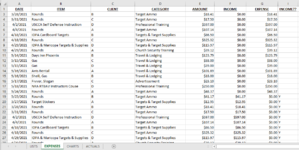
1. I'm at work, and IT does not allow add-ins, so I can't use the XL2BB add-in to share my data. I have included a screen capture of most of my range.
2. Because this is being created for others who for reasons unknown want it "this way!", columns F and G would normally be hidden. The user would complete columns A through E (C and D are Data Validation drop-down lists, and then if the AMOUNT value is to be considered income, puts a Y in column I; formulas then pull the value into either F or G. Column H is blank and hidden to create a buffer between the range/table data and everything else.
3. This is a test book, so I simply copied the existing entries and entered the Y down column I. A real workbook would not have duplicate entries and values - hopefully!!

When using the search for pivot tables with a dynamic range, every answer used VBA. I'd rather try to stay away from VBA for this one. Can someone please drop-kick me in a good direction for this one??
I am new to Pivot Tables. I used the built-in wizards to create a pivot from a named table with a static range. Unfortunately - but I should have expected it, when I tried to insert a row of data in the middle of the table, I got an error that said I couldn't do that because it would change my table. I'm assuming that's due to (A) having a static defined range, and (B) having a connected Pivot Table??
So I thought if I simply used a dynamic range as the data source for my pivot, all should be good. My data is on a sheet named EXPENSES, from columns A to G; headers in row 1, data currently down to row 37. All my column headers are single word, with no spaces, numbers, special characters, or punctuation. I can define the table MyExpenses with RefersTo formula =OFFSET(EXPENSES!$A$1,1,0,COUNTA(EXPENSES!$G:$G),7).
On a sheet named CHARTS, I select B2 and attempt INSERT >> Pivot Table. But when I enter MyExpenses for the Table/Range, I get this error:
"The PivotTable field name is not valid. To create a Pivot Table report, you must use data that is organized as a list with labeled columns. If you are changing the name of a Pivot Table field, you must type a new name for the field." I also tried entering the OFFSET formula directly as the Table/Range, but got "Data source reference is not valid."
Three notes:
1. I'm at work, and IT does not allow add-ins, so I can't use the XL2BB add-in to share my data. I have included a screen capture of most of my range.
2. Because this is being created for others who for reasons unknown want it "this way!", columns F and G would normally be hidden. The user would complete columns A through E (C and D are Data Validation drop-down lists, and then if the AMOUNT value is to be considered income, puts a Y in column I; formulas then pull the value into either F or G. Column H is blank and hidden to create a buffer between the range/table data and everything else.
3. This is a test book, so I simply copied the existing entries and entered the Y down column I. A real workbook would not have duplicate entries and values - hopefully!!

When using the search for pivot tables with a dynamic range, every answer used VBA. I'd rather try to stay away from VBA for this one. Can someone please drop-kick me in a good direction for this one??


