Create shapes based on filtered rows in a table

[liberovago]

Good afternooneveryone!!!

I would need to automate the process of creating rectangles.

So:

I have a table (where there are rows that change from week to week, some are deleted, and some are added). Of the rows I add, I should create rectangles, and then export them to other sheets.

Before and after this process there are already a whole series of macros that help me; at the moment the operation I described, I do it manually. But I would like to automate it.

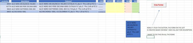
So I have this table, which I filter based on the newly created rows (which are products): I would like a macro to create rectangles for me, and as the text in the rectangle, comes a link to the cell where there is a description of that product. Example the form "Rectangle6" in the formula bar has =G!BA78 (G is the name of the sheet, ba78 where there is the text that is to be displayed).

The problem is that when I filter the table, I don't know how to proceed, in the sense that out of the whole table, I only have a few rows of new products. I don't know how to tell it "create a rectangle of the first filtered row displayed (example row #7), then create a rectangle of the second filtered row displayed (example row #14), and so on.

A first step with code I sketched it out, and the first rectangle I can create. But then I don't know how to continue, because if I change the references, to my current knowledge, he creates the rectangle after me at the next row of the table, but not the displayed row, but the row of the whole table...

The code is this

Sub CreateForms()
      
    ' Define the range of the filtered table
    Dim tblRange As Range
    Set tblRange = Range("Tabella4")

    ' Get the filtered rows of the table
    Dim tblRows As Range
    Set tblRows = tblRange.SpecialCells(xlCellTypeVisible)

    ' Define the cell that contains the formula
    Dim formulacell As Range
    Set formulacell = tblRows(1, 52).Offset(0, 1)

    ' Define the position and size of the shape
    Dim shapeLeft As Double
    shapeLeft = tblRange.Left + tblRange.Width + 10 ' 10 is the gap between the table and the shape
    Dim shapeTop As Double
    shapeTop = tblRange.Top
    Dim shapeWidth As Double
    shapeWidth = 100
    Dim shapeHeight As Double
    shapeHeight = 50

    ' Add the shape to the worksheet
    Dim shape As shape
    Set shape = ActiveSheet.Shapes.AddShape(msoShapeRectangle, shapeLeft, shapeTop, shapeWidth, shapeHeight)

    ' Set the formula of the shape to the formula in the cell
    shape.DrawingObject.Formula = "=G!" & formulacell.Address(True, True, xlA1, External:=False)
    
End Sub

Sorry for my English!