Create signal using conditional formatting

Lolipop

New Member
Joined
May 24, 2023
Messages
5
Office Version
  1. 365
Platform
  1. Windows
Hi!

I have question regarding the conditional formatting. How to show signal using conditional formatting icon set?

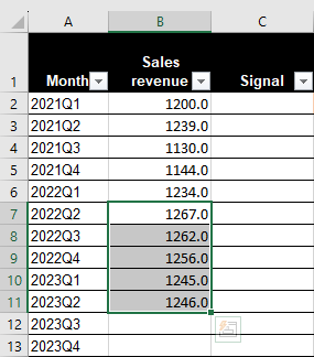
I'm planning to make a signal when the 3 or 5 value is showing nearest value among them (example in the picture), then the signal will show red flag in C11. The thing is the value is not fixed. So, how can I set the conditional formatting?

Thank you in advance.

medium
 

Excel Facts

Format cells as date
Select range and press Ctrl+Shift+3 to format cells as date. (Shift 3 is the # sign which sort of looks like a small calendar).
Please don't use a picture to display your data. Use XL2BB so that no one has to retype your information.

Also, what do you mean the "3 or 5 value" ?
It would be helpful if you showed some form of expected result(s) when you use XL2BB.
 
Upvote 0
Welcome to the Mr. Excel forum.
But, I'm unsure of your question. What do you mean by Signal?

Can you use the xl2bb add in (link below) to share a mini workbook?

Please post an example of what "the 3 or 5 value is showing nearest value among them" means?
 
Upvote 0
Sorry for the inconvenience caused. I cant use XL2BB as there is some problem occurred.
Here is the scenario. I created a graph showing the trend of the data. As you can see the circle in the graph, there is 3 to 5 value/point that show steady line which is a sign that the natural limit need to recalculate in order to achieve the target. So, how can I tell/notify the user that the natural limit need to be recalculate? My idea is I want to put the sign in the signal column to inform user that at certain point, user need to recalculate their natural limit or need to investigate unusual trend. When user see there is red flag in signal column they know what they should do. The question is how to create conditional formatting using icon in signal column? What formula should I use?

FYI, red flag icon represent sign that the natural limit need to be recalculate or need to investigate unusual trend.

1685000738108.png
 
Upvote 0
Okay, so you want to know when Column B exceeds some value.
What column is that value in? Why is 2023Q2 flagged but the 2021Q2, 2022Q1-2023Q1 not flagged?

We need more information.
 
Upvote 0
I created the following:

*excel formulas are in table format. You said 3 to 5 to make a trend. I chose the past 4. Column H calculates the past 4 move averages. And Column J calculates the average deviation from central line.

With that, column C Signal, checks if (Past 4 Move Average/Sales revenue) is less than or equal to 2%, adjust 2% as needed depending on what you think is a small deviation.

Similarly, also checks if deviation from central line is greater than or equal to 3%, adjust 3% as needed depending on what you think is a big enough deviation to investigate.

Good luck!

Test.xlsx
ABCDEFGHIJ
1QuarterSales revenueSignalCentralNatural Process LimitNatural Process Limit UpperMoving RangePast 4 Move AveragePast 4 AverageAverage Deviation from Central Line
22021Q11200 1202.351050.713540000
32021Q21239 1202.351050.7135439000
42021Q31130 1202.351050.7135410949.333333331189.666667-12.68333333
52021Q41144 1202.351050.713541440.51178.25-24.1
62022Q11234 1202.351050.7135490631186.75-15.6
72022Q21267 1202.351050.713543361.51193.75-8.6
82022Q31262 1202.351050.71354535.51226.7524.4
92022Q41256 1202.351050.71354633.51254.7552.4
102023Q11245Investigate1202.351050.713541113.751257.555.15
112023Q21246Investigate1202.351050.7135415.751252.2549.9
122023Q3 1202.351050.7135404.5124946.65
132023Q4 1202.351050.71354031245.543.15
Sheet1
Cell Formulas
RangeFormula
C2:C13C2=IF(AND(IFERROR([@[Past 4 Move Average]]/[@[Sales revenue]],1)<=0.02,IFERROR(ABS([@[Average Deviation from Central Line]]/[@[Sales revenue]])>=0.03,1)),"Investigate","")
D2:D13D2=AVERAGE(Table1[@[Natural Process Limit]:[Natural Process Limit Upper]])
G2:G13G2=IF([@[Sales revenue]]<>"",IFERROR(ABS([@[Sales revenue]]-OFFSET([@[Sales revenue]],-1,)),0),0)
H2:H13H2=IFERROR(AVERAGE([@[Moving Range]]:OFFSET([@[Moving Range]],-3,)),0)
I2:I13I2=IFERROR(AVERAGE([@[Sales revenue]]:OFFSET([@[Sales revenue]],-3,)),0)
J2:J13J2=IF([@[Past 4 Average]]=0,0,[@[Past 4 Average]]-[@Central])
 
Upvote 0

Forum statistics

Threads
1,214,827
Messages
6,121,818
Members
449,049
Latest member
cybersurfer5000

We've detected that you are using an adblocker.

We have a great community of people providing Excel help here, but the hosting costs are enormous. You can help keep this site running by allowing ads on MrExcel.com.
Allow Ads at MrExcel

Which adblocker are you using?

Disable AdBlock

Follow these easy steps to disable AdBlock

1)Click on the icon in the browser’s toolbar.
2)Click on the icon in the browser’s toolbar.
2)Click on the "Pause on this site" option.
Go back

Disable AdBlock Plus

Follow these easy steps to disable AdBlock Plus

1)Click on the icon in the browser’s toolbar.
2)Click on the toggle to disable it for "mrexcel.com".
Go back

Disable uBlock Origin

Follow these easy steps to disable uBlock Origin

1)Click on the icon in the browser’s toolbar.
2)Click on the "Power" button.
3)Click on the "Refresh" button.
Go back

Disable uBlock

Follow these easy steps to disable uBlock

1)Click on the icon in the browser’s toolbar.
2)Click on the "Power" button.
3)Click on the "Refresh" button.
Go back
Back
Top