Creating 2 linked drop downs

[hungledink]

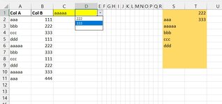
I have some data, names in column A and corresponding account number in column B.

I've made a drop-down lists with data validation, one in cell C1 for the data in column A, and in D1 for data in column B.

Is it possible to have it so that if a selection is made in cell C1, a selection from column A, then the value in cell D1 will auto populate with the corresponding value from column B and vice versa?

 

[Automatrix]

Not really. If you choose a value from the dropdown, it will overwrite the formula. But you can add an adjacent "suggestion" cell with the value using XLOOKUP.

Book4
	A	B	C	D	E
1	Name	Account		NameList	AccountList
2	Adam	Adam-1		Adam	Adam-1
3	Bob	Bob-1		Bob	Bob-1
4	Carol	Carol-1		Carol	Carol-1
5
6	Enter name	Adam
7	Suggested name
8
9	Enter account number
10	Suggested account	Adam-1
Sheet1

Cell Formulas
Range	Formula
D2:D4	D2	=Data[Name]
E2:E4	E2	=Data[Account]
B7	B7	=XLOOKUP(B9,Data[Account],Data[Name],"")
B10	B10	=XLOOKUP(B6,Data[Name],Data[Account],"")
Dynamic array formulas.

Cells with Data Validation
Cell	Allow	Criteria
B6	List	=$D$2#
B9	List	=$E$2#

Columns D and E contain dynamic arrays in order to update the dropdown list as new names are added to the data table. They can be hidden or placed in another sheet.

 

[Anthony47]

Don't know whether the proposal from @Automatrix solve your problem.

If Not, then you might try the following (requires XL 365 or other Dynamic array compliant versions):
-create in S1 a first list using the formula

=LET(dColA;A2:A15;dColB;B2:B15;fVal;D1;fArr;SE(fVal="";SE(dColA<>"";dColA;""); SE(dColB=fVal;dColA;""));DATI.ORDINA(UNICI(fArr)))

-create the second list in T1 using the formula

=LET(dColA;A2:A15;dColB;B2:B15;fVal;D1;fArr;SE(fVal="";SE(dColA<>"";dColA;""); SE(dColB=fVal;dColA;""));DATI.ORDINA(UNICI(fArr)))

Now set the data validation for C1 using as source of the list the formula =S1#
Repeat for D1 using the formula =T1#

See the attached image to see how the validation lists changes in my test sheet

Then try and see how this behave for you

 

[darkhangelsk]

Don't know whether the proposal from @Automatrix solve your problem.

If Not, then you might try the following (requires XL 365 or other Dynamic array compliant versions):
-create in S1 a first list using the formula

=LET(dColA;A2:A15;dColB;B2:B15;fVal;D1;fArr;SE(fVal="";SE(dColA<>"";dColA;""); SE(dColB=fVal;dColA;""));DATI.ORDINA(UNICI(fArr)))

-create the second list in T1 using the formula

=LET(dColA;A2:A15;dColB;B2:B15;fVal;D1;fArr;SE(fVal="";SE(dColA<>"";dColA;""); SE(dColB=fVal;dColA;""));DATI.ORDINA(UNICI(fArr)))

Now set the data validation for C1 using as source of the list the formula =S1#
Repeat for D1 using the formula =T1#

See the attached image to see how the validation lists changes in my test sheet

Then try and see how this behave for you

can i request an example sheet? this might be an answer to my question as i have long list and the data available could go to 'Account' or 'Name' and if it is possible to have a 3rd selection. Thank you!

 

[Anthony47]

A demo file can be downloaded from here: CrossValidation.xlsx

You need to modify the formulas in S1-T1 if the list in columns A-B is longer than 20 lines
Data validation is set in cells C1-D1