Creating a Double Axis Dynamic Chart with Four Tables and a Drop Down Selection

[tmed834]

Hello, this is my first post! Pleasure to join the forum.

So I am trying to create a double axis chart, one will be a bar chart and the other will be a line chart. I have four locations I want to do this for, but if I have the data for all four countries then the visuals will be way too crammed. Here is some of the data below:

Date	Australia Conversions	Australia CPA	Hong Kong Conversions	Hong Kong CPA	New Zealand Conversions	New Zealand CPA	SingaporeConversions	Singapore CPA
8/1/2009	10	27.259	4	15.5675	4	23.4875	21	9.514285714
8/2/2009	11	31.68181818	1	67.57	4	47.445	10	23.264

<colgroup><col><col><col><col><col><col><col><col><col></colgroup><tbody>
</tbody>

And here is the chart for just one of the tables (one table for each country).

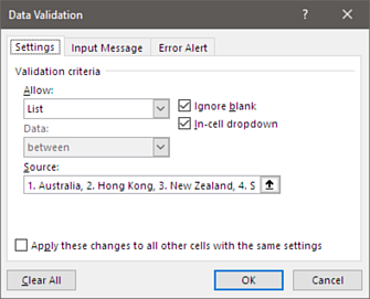
Essentially, if I can have a drop down list above the legend, where I can choose either Australia, Singapore, Hong Kong or New Zealand, then someone viewing the chart can have all the data here and select accordingly.

Thanks, and apologies if I broke any rules in how I posted. I read the rules, but not entirely. I will fix the thread if there is something blatantly wrong.

 

[thisoldman]

I haven't seen your complete data set. From what you show in the one chart, you might see better separation of the blue bars and the red line if you uses a single 0–70 vertical scale.

A different, separate cell range from the original data range is used for the chart source data.

I plotted some random or dummy data in T5:AB66. The headers were in row 5, dates in column T, SG CPAs in column AB.

The chart source data was in B5:D66. Column B just duplicates the dates in column T.

I put a Data Validation dropdown box in G3. Settings were for Allow: List; Source: 1. Australia,2. Hong Kong,3. New Zealand,4. Singapore
The numbers in the Data Validation Source list allow us to copy the values from the original data block to the charted data block using a CHOOSE formula rather than an INDEX+MATCH, VLOOKUP, or nested IF formula.

The charted data:

	B	C	D
5	Date	NZ Conversions	NZ CPA
6	08/01/2009	11	47.905
7	08/02/2009	11	31.708
8	08/03/2009	34	8.196
9	08/04/2009	12	8.153

<tbody>
</tbody>

Formula in C5, copied to the right and downward:
=CHOOSE(LEFT($G$3),U5,W5,Y5,AA5)

My example file is available at https://www.dropbox.com/s/vfv615swlgvtkf3/dynamic_chart_for_tmed834.xlsx?dl=0

 

[tmed834]

I haven't seen your complete data set. From what you show in the one chart, you might see better separation of the blue bars and the red line if you uses a single 0–70 vertical scale.

A different, separate cell range from the original data range is used for the chart source data.

I plotted some random or dummy data in T5:AB66. The headers were in row 5, dates in column T, SG CPAs in column AB.

The chart source data was in B5:D66. Column B just duplicates the dates in column T.

I put a Data Validation dropdown box in G3. Settings were for Allow: List; Source: 1. Australia,2. Hong Kong,3. New Zealand,4. Singapore
The numbers in the Data Validation Source list allow us to copy the values from the original data block to the charted data block using a CHOOSE formula rather than an INDEX+MATCH, VLOOKUP, or nested IF formula.

The charted data:

	B	C	D
5	Date	NZ Conversions	NZ CPA
6	08/01/2009	11	47.905
7	08/02/2009	11	31.708
8	08/03/2009	34	8.196
9	08/04/2009	12	8.153

<tbody>
</tbody>

Formula in C5, copied to the right and downward:
=CHOOSE(LEFT($G$3),U5,W5,Y5,AA5)

My example file is available at https://www.dropbox.com/s/vfv615swlgvtkf3/dynamic_chart_for_tmed834.xlsx?dl=0

Amazing!!!!!!! This is exactly what I wanted. I never really used the data validation tool or the choose formula at my last job, so I need some more practice with those. But I will use your example and study it so I can replicate this in the future. But your explanation is great.

Thanks so much!

 

[thisoldman]

Thanks for the kind words. You made me smile for much of the day.

 

[tmed834]

Thanks for the kind words. You made me smile for much of the day.

Haha. No problem. Thanks again!!